Text Analysis of NHL Hockey Coach Interviews

Collecting Data - The 2016 Stanley Cup Final

The 2016 Stanley Cup Final series took place between May 30 and June 12 of 2016. The Penguins won Games 1 and 2, the latter in overtime, to take a 2-1 series lead. The Sharks and Penguins then alternated wins, with the Penguins taking Game 6 to clinch the Stanley Cup (all info from Hockey Reference).

We will scrape the pre- and post-game interview transcripts from ASAP Sports, which hosts a collection of transcripts from various sporting events. The remainder of this section, describing the scraper used to collect the transcript texts, is admittedly a little code heavy (though I still might expand on it further in a separate post). For those who want the data handy to play along without scraping, you can download the data directly from my Github. If you want to skip directly to the text analysis, click here.

Navigating to the 2016 Stanley Cup Final page, we see a collection of links for each day of the series. Each of these links leads to a set of additional links, which each contain an interview with a player, coach or other important figure.

get.transcripts <- function(url){
  
  urls <- read_html(url) %>% 
    html_nodes("a") %>%
    html_attr("href") # Extract the url attributes
  
  # Relevant links have the 'show_interview.php?' tag
  relevant.urls <- urls[grepl(urls,pattern="show_interview.php?",fixed=T)] 
  
  # Run text extraction function on each link
  transcripts <- rbind.fill(map(relevant.urls,extract.interview.text))
  
  return(transcripts)
}


extract.interview.text <- function(url){
  
  text <- read_html(url) %>%
    html_nodes("td") %>% 
    html_text() # Extract text
  
  # Relevant text 
  text.clean <- text[grepl(text,pattern="FastScripts Transcript by ASAP Sports",fixed=T)]
  
  # Split information into separate strings, remove whitespace at the beginning and end of each
  text.clean.split <- str_trim(str_split(text.clean,pattern="\n")[[2]])
  
  # Remove empty strings, remove the ASAP sports tag from strings
  raw.text <- gsub(text.clean.split[text.clean.split != ""],pattern=" FastScripts Transcript by ASAP Sports",replacement="")
  
  # Extract date (in second string)
  date <- mdy(raw.text[2])
  
  # Third string contains the interview subject, though everything is squashed together
  # Put spaces between capital letters, split based on whitespace, then combine the second and fourth token as the subject
  tokens <- unlist(strsplit(gsub('([[:upper:]])',' \\1',raw.text[3]),"[[:space:]]"))
  subject <- paste(tokens[2],tokens[4])
  
  # Find index of the string where the interview starts, which is the first string where 'Q.' and 'MODERATOR' serves as a prompt
  # For interviews taking place after games, there is additional text in the preamble. Therefore, if this index is large, we can infer this is a post-game interview 
  interview.starts <- min(c(which(str_detect(raw.text,"Q.")),which(str_detect(raw.text,"MODERATOR"))))
  after.game <- interview.starts > 4
  
  # Actual text is from the above found index onward
  interview.text <- raw.text[interview.starts:length(raw.text)]
  
  # Remove general prompts
  relevant.interview.text <- paste(interview.text[!str_detect(interview.text,"Q.") & !str_detect(interview.text,"MODERATOR")],collapse=" ")
  
  # Combine information into data frame
  interview.data <- data.frame(Date=date,Subject=subject,AfterGame=after.game,Text=relevant.interview.text,stringsAsFactors=F)
  
  return(interview.data)
  
}

The scraper makes use of the read_html function from Hadley Wickham’s rvest package to extract the html from the desired web pages. We then parse the html based on the relevant css selector using html_nodes. For example, the relevant parts of the page containing interview links will begin with <a href=...>. Finally, we extract our desired information using either the html_attrs or html_text functions. See the comments in the above code, or the documentation for some more information.

We first extract all the links from the main web page. The links we are interested in are those for the individual games, which can be identified with the show_event.php? tag. We run the get.transcripts function on each of these links. This function will load the page, then collect the links representing each of the interviews (in this case, they can be identified by the show_interview.php? tag). Then the extract.interview.text function is run on each of these links, which loads the page, extracts the text, and collects some other relevant information, such as the date and the subject of the interview. Again, the comments in the above code provide some clarification.

cup.final.url <- paste0("http://www.asapsports.com/show_events.php?category=5&year=2016&title=NHL+STANLEY+CUP+FINAL%3A+SHARKS+v+PENGUINS")

# Extract links
transcript.urls <- read_html(cup.final.url) %>%
  html_nodes("a") %>%
  html_attr("href")

# Relevant links have the 'show_event.php?' tag
relevant.transcript.urls <- transcript.urls[grepl(transcript.urls,pattern="show_event.php?",fixed=T)]

# Run function on links
transcripts <- rbind.fill(map(relevant.transcript.urls,get.transcripts)) %>%
  mutate(Subject = gsub(Subject,pattern="Peter De",replacement="Peter DeBoer"))

Basic Text Analysis

Let’s get a general sense of our data. First, our text requires a few more steps of cleaning before being ready for analysis. Since our scraper collected all of the interviews available over the course of the Cup Final, we filter out all the non-coach interviews, so that our sujects are only ‘Mike Sullivan’ or ‘Peter DeBoer’. We remove the prompts from the text, and create a single label with the date and whether the interview took place after a game or not; this label will be useful later. Then, using the unnest_tokens function from the tidytext package, we extract each word from the text onto its own row in a new data frame, then filter out all the ‘stop words’ (common words that don’t provide any meaningful information, such as prepositions and conjunctions). The list of stop words is available through the stop_words data frame from the tidytext package.

# Focus on interviews with either coach Mike Sullivan or Peter DeBoer, remove prompts from text,
# and add label to interview

label.function <- function(Date,AfterGame){
  return(ifelse(AfterGame,paste(Date,"Post-Game"),Date))
}

coaches.text <- transcript %>% 
  filter(Subject %in% c("Mike Sullivan","Peter DeBoer")) %>%
  mutate(Text = gsub(Text,pattern="COACH SULLIVAN: ",replacement="")) %>%
  mutate(Text = gsub(Text,pattern="COACH DeBOER: ",replacement="")) %>%
  rowwise() %>%
  mutate(Label = label.function(Date,AfterGame)) %>%
  ungroup()
  

# Split text into words, filter out 'stop words'
coaches.words <- coaches.text %>%
  unnest_tokens(Word,Text) %>%
  filter(! Word %in% stop_words$word)

head(coaches.words,n=12)

## # A tibble: 12 x 5
##          Date       Subject AfterGame                Label       Word
##         <chr>         <chr>     <lgl>                <chr>      <chr>
##  1 2016-06-12 Mike Sullivan      TRUE 2016-06-12 Post-Game      learn
##  2 2016-06-12 Mike Sullivan      TRUE 2016-06-12 Post-Game        lot
##  3 2016-06-12 Mike Sullivan      TRUE 2016-06-12 Post-Game      learn
##  4 2016-06-12 Mike Sullivan      TRUE 2016-06-12 Post-Game        lot
##  5 2016-06-12 Mike Sullivan      TRUE 2016-06-12 Post-Game    process
##  6 2016-06-12 Mike Sullivan      TRUE 2016-06-12 Post-Game     people
##  7 2016-06-12 Mike Sullivan      TRUE 2016-06-12 Post-Game   business
##  8 2016-06-12 Mike Sullivan      TRUE 2016-06-12 Post-Game   coaching
##  9 2016-06-12 Mike Sullivan      TRUE 2016-06-12 Post-Game    players
## 10 2016-06-12 Mike Sullivan      TRUE 2016-06-12 Post-Game management
## 11 2016-06-12 Mike Sullivan      TRUE 2016-06-12 Post-Game   scouting
## 12 2016-06-12 Mike Sullivan      TRUE 2016-06-12 Post-Game     people

Let’s make a simple display of the 20 most common words used by each coach and their frequency. We can also make word clouds to display the most common words used by each coach. Note that legends are omitted in some of the plots going forward. Gold coloring refers to Mike Sullivan of the Pittsburgh Penguins, while teal refers to Peter DeBoer of the San Jose Sharks.

## Most Common Words

# Count individual occurrences of each word
coaches.word.count <- coaches.words %>%
  count(Word,Subject) %>%
  ungroup() %>%
  group_by(Subject) %>%
  top_n(20) %>%
  rename(Occurrences = n)

# Set team colors
team.colors <- c("#c5b358","#007889") # Pittsburgh Gold and San Jose Teal respectively
  
# Plots of 20 most common words by coach
ggplot(data=coaches.word.count,aes(x=Word,y=Occurrences,fill=Subject)) +
  facet_wrap(~Subject, scales="free_y") +
  geom_bar(stat="identity",show.legend=F) +
  scale_fill_manual(values=team.colors) +
  xlab("Word") +
  coord_flip() +
  theme_bw(15)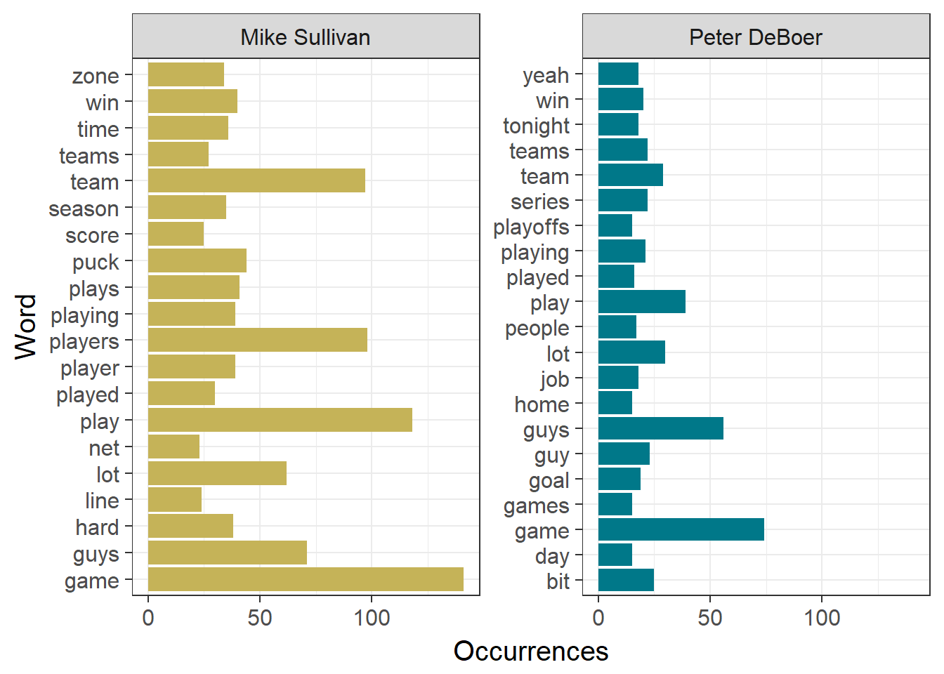

# Word clouds for each coach
coaches.words %>%
  filter(Subject == "Mike Sullivan") %>%
  count(Word) %>%
  with(wordcloud(Word,n,max.words=100,colors=team.colors[1]))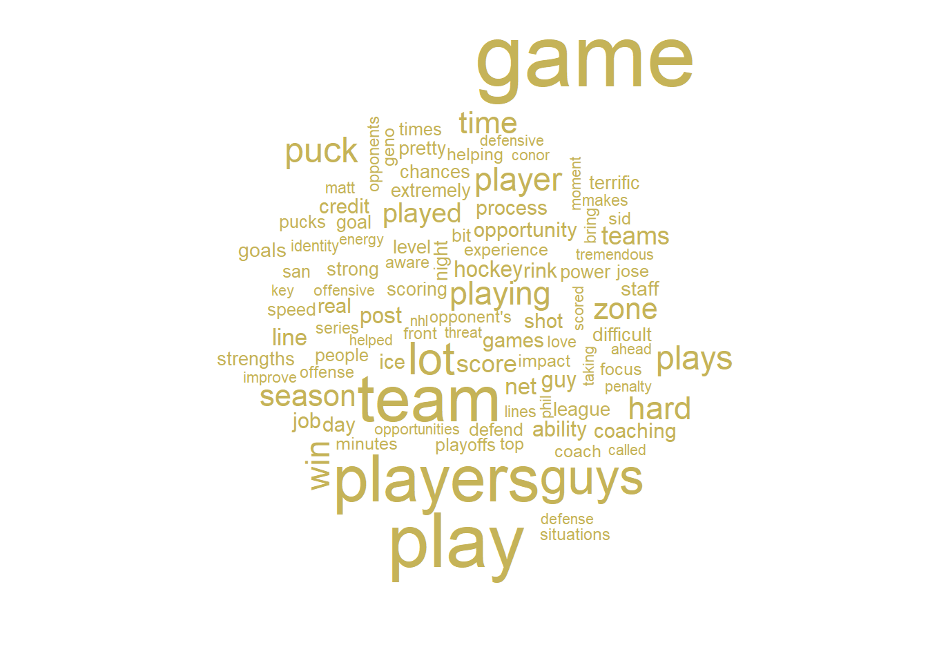

coaches.words %>%
  filter(Subject == "Peter DeBoer") %>%
  count(Word) %>%
  with(wordcloud(Word,n,max.words=100,colors=team.colors[2]))

These words are more or less what you would expect a hockey coach to be saying in an interview. The most frequent word used by each coach is ‘game’, and they both use several derivatives of the word ‘play’. There are also plenty of references to hockey-specific subjects, such as ‘puck’ and ‘net’. All in all, no real surprises (or insight) here.

Let’s see if we can find any differences between the speaking patterns of these two coaches. This first technique is the same used by David Robinson in his Trump post. For each word, we compare the frequency of use by Sullivan to that of DeBoer by taking the natural log of their ratio. High positive values refer to words used more frequently by Sullivan, while negative values refer to words used more frequently by DeBoer.

## Most Different Words

coach.ratios <- coaches.words %>%
  count(Word,Subject) %>%
  rename(Occurrences = n) %>%
  filter(sum(Occurrences) > 5) %>% # Focus on words appearing at least 5 times in the text
  spread(Subject,Occurrences,fill=0) %>%
  ungroup() %>%
  mutate_each(funs((. + 1) / sum(. + 1)), -Word) %>% # Fraction of word usage by each coach
  mutate(LogRatio = log2(`Mike Sullivan`/`Peter DeBoer`)) %>%
  arrange(LogRatio) %>%
  group_by(LogRatio > 0) %>%
  mutate(Team = ifelse(LogRatio > 0,"Pittsburgh","San Jose")) %>%
  top_n(10, abs(LogRatio)) %>% # Get top 10 words in each direction
  ungroup()

# Plot of top 10 words most often used by each coach relative to the other
ggplot(data=coach.ratios,aes(x=reorder(Word,LogRatio),y=LogRatio,fill=Team)) +
  geom_bar(stat="identity",show.legend=F) +
  scale_fill_manual(values=team.colors) +
  xlab("Word") +
  ylab("Log Ratio (Sullivan vs. DeBoer)") +
  coord_flip() +
  theme_bw(15)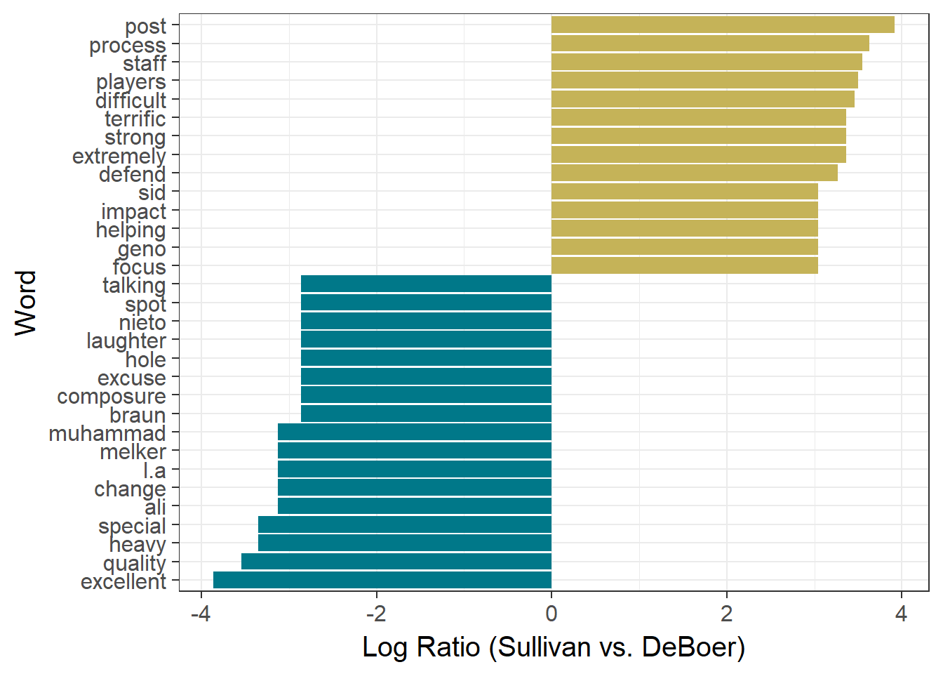

Results here are largely uninteresting, with both coaches employing a smattering of different hockey-centric words and qualifiers. Of the few standout words, we should probably expect Sullivan to refer to his players ‘Sid’ and ‘Geno’ more often than his counterpart, and DeBoer to refer to his opponent as ‘Pittsburgh’.

Another way to make the comparision between the coaches is by calculating the tf-idf for each word. This value is obtained by multiplying the term frequency, the fraction of occurrences of the word in the text, by the inverse document frequency, the log of the ratio of the total number of ‘documents’ to the number of documents in which the word in question appears. This value is higher for words that appear more sparingly across documents. For this analysis, if we only considered the two sets of texts provided by each coach as the two documents, we would only obtain two possible values for tf-idf, one of which being 0. Instead, we will split the text by individual interview, then recombine the top words for each interview by coach in the plot.

# TF-IDF

# Number of occurences of each word by interview
all.coaches.words <- coaches.words %>%
  count(Subject,Word,Label,sort=T) %>%
  ungroup()

# Total words per interview
total.words <- coaches.words %>%
  count(Subject, Label) %>%
  ungroup()

# Get top words by TF-IDF for each interview
top.words.tf <- left_join(all.coaches.words,total.words,by=c("Subject","Label")) %>%
  rename(Occurrences=n.x,Total=n.y) %>%
  mutate(Document = paste(Subject,Label)) %>% # Merge subject and label for use in bind_tf_idf function
  bind_tf_idf(Word,Document,Occurrences) %>%
  arrange(desc(tf_idf)) %>%
  mutate(Word = factor(Word, levels = rev(unique(Word)))) %>%
  group_by(Document,Label) %>% 
  top_n(1) %>% 
  ungroup()

ggplot(top.words.tf, aes(Word, tf_idf, fill = Subject)) +
  geom_bar(stat = "identity", show.legend = F) +
  facet_wrap(~Subject, ncol = 2, scales = "free_y") +
  scale_fill_manual(values = team.colors) +
  ylab("tf-idf") +
  coord_flip() + 
  theme_bw(15)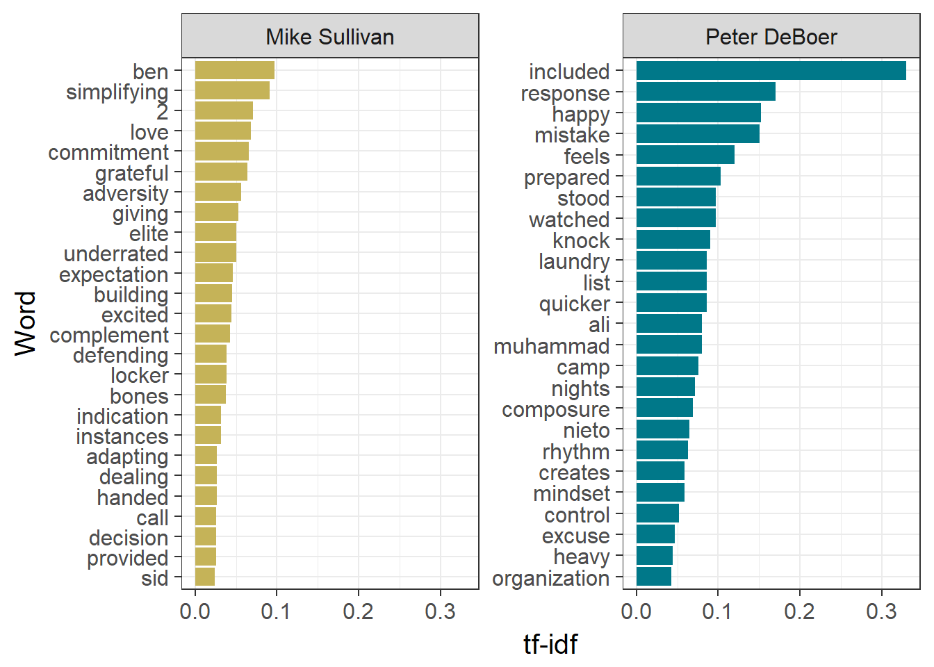

Notice that there are fewer hockey-centric terms here, as these would probably be used in many of the interviews. We find some references to coaches’ own players again (including Long Beach Native™ Matt Nieto), along with a reminder that I should have removed individual numbers from the text before running the analyses (my bad!). Otherwise, we get a small glimpse into the mindset of each coach, with Sullivan using words like ‘commitment’, ‘expectation’, ‘adapting’, and DeBoer using words like ‘composure’, ‘rythym’, and ‘control’

Through DeBoer’s words we also get a reminder that Muhammad Ali had passed away while this series took place. RIP.

Sentiment Analysis

We can apply sentiment analysis techniques to the interviews to get an idea of the mindset of the coaches over the course of the series. A number of sentiment lexicons, associating individual words to emotions or feelings, are available through the tidytext package. We first use the NRC Word-Emotion Association Lexicon, which categorizes each word into a number of categories (positive, negative, anger, anticipation, disgust, fear, joy, sadness, surprise, and trust). Here’s a snippet to get a sense of the nrc lexicon.

## Sentiment Categories

# Prepare sentiment dataset
nrc <- sentiments %>%
  filter(lexicon == "nrc") %>%
  select(word, sentiment) %>%
  rename(Word = word, Sentiment = sentiment)

head(nrc)

## # A tibble: 6 x 2
##        Word Sentiment
##       <chr>     <chr>
## 1    abacus     trust
## 2   abandon      fear
## 3   abandon  negative
## 4   abandon   sadness
## 5 abandoned     anger
## 6 abandoned      fear

We count for each coach the frequency of words falling under each sentiment category and then plot the sentiment over time. This is done my using inner_join from the dplyr package to merge in the sentiment information from the nrc lexicon to the words in the coach text.

# Count the total number of words used by each coach each interview
coaches.words.by.interview <- coaches.words %>%
  group_by(Subject,Label) %>%
  mutate(TotalWords = n()) %>%
  ungroup() %>%
  distinct(Subject, Label, TotalWords)

coaches.word.by.sentiment <- coaches.words %>%
  inner_join(nrc, by = "Word") %>%
  count(Sentiment,Label,Subject) %>% # Count occurrences of each word by each coach in each interview
  rename(Occurrences = n) %>%
  inner_join(coaches.words.by.interview, by = c("Label","Subject")) %>% # Merge total words
  mutate(Frequency = Occurrences/TotalWords)

# Plot the sentiment trajectories over time
ggplot(data=coaches.word.by.sentiment,aes(x=Label,y=Frequency,color=Subject, group=Subject)) +
  facet_wrap(~Sentiment, nrow=5) +
  geom_line(show.legend=F) +
  geom_point(show.legend=F) +
  scale_color_manual(values = team.colors) +
  xlab("Interview") +
  theme_bw(15) +
  theme(axis.text.x = element_text(angle=90))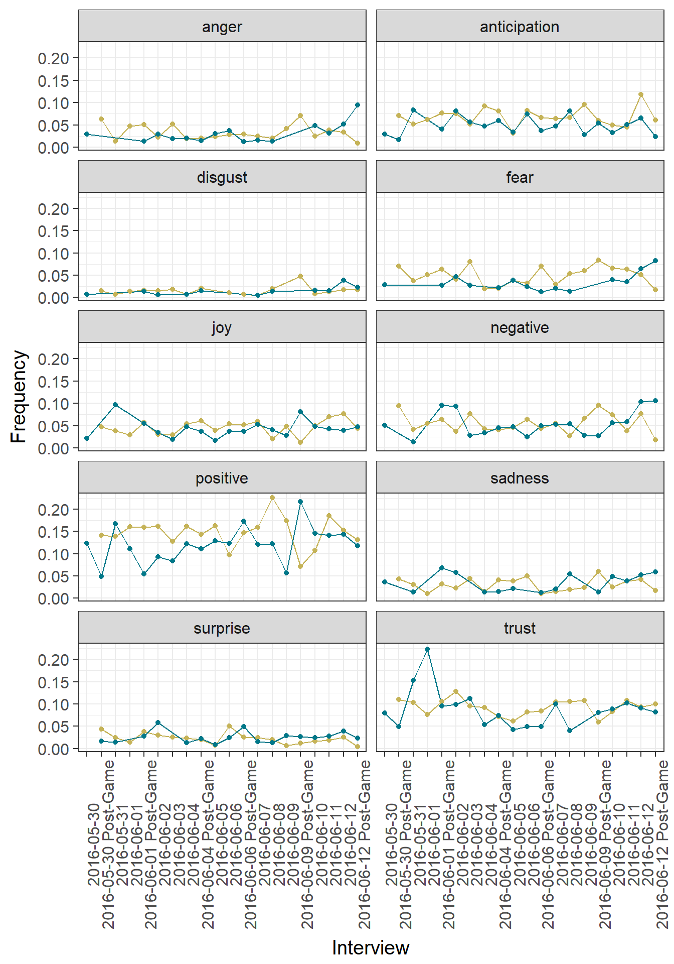

Notice the high positivity from Pittsburgh’s Sullivan in the days following Game 4 (after going up 3 games to 1) and San Jose’s DeBoer after Game 5 (a win that staved off elimination). Also check out the spike in trust in the days following the Game 1 loss by the Sharks, which may reflect DeBoer rallying his troops for an important Game 2. We can see spikes in anticipation for Sullivan before (what turned out to be) the decisive Game 6. On the other hand, there is a small spike in anger for DeBoer after losing the Stanley Cup (understandable!).

Alternatively, we can simplify analysis and look at the difference between positive and negative words used by each coach over time. Here we use Bing Liu’s lexicon, which categorizes words simply as positive or negative.

## Positive vs. Negative

# Get top 10 positive and negative words used by each coach and plot
sentiment.words <- coaches.words %>%
  inner_join(get_sentiments("bing"), by=c("Word"="word")) %>%
  rename(Sentiment = sentiment) %>%
  count(Word,Subject,Sentiment,sort=T) %>%
  ungroup() %>%
  group_by(Subject,Sentiment) %>%
  top_n(10) %>%
  rename(Occurrences = n)  %>%
  arrange(Subject,Sentiment,Word)

ggplot(data=sentiment.words,aes(x=reorder(factor(Word),Occurrences),y=Occurrences,fill=Subject)) +
  geom_bar(stat="identity",show.legend=F) +
  facet_wrap(~Sentiment + Subject, scales="free_y") +
  scale_fill_manual(values = team.colors) +
  xlab("Word") +
  coord_flip() +
  theme_bw(15)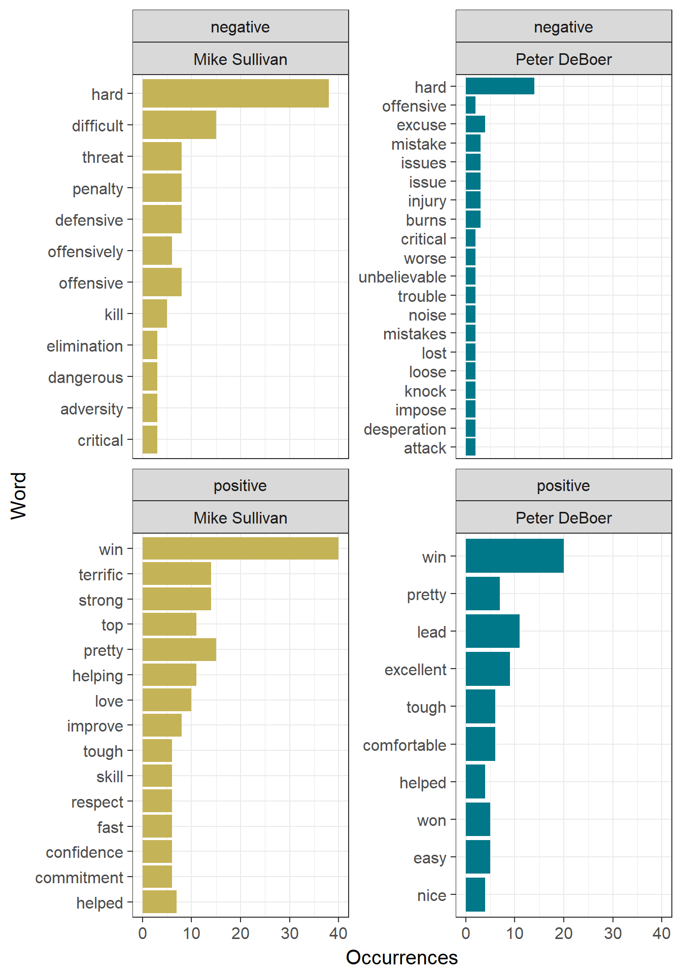

In general, nothing unexpected here. The most positive word for each coach is ‘win’. Here we see how tricky text analysis can be in most cases. For example, ‘hard’, the most often used negative word by each coach, probably refers to ‘playing hard’, which in a hockey context, should in fact be considerd as a positive. Also, some hockey specific words have their meaning distorted in this lexicon, such as ‘kill’, which in this context refers to penalty kills. Finally, ‘burns’ in this case refers to Brent Burns, and is almost certainly not a negative; in fact, he was a Norris finalist that season!

Keeping that in mind, we plot the positivity of each coach over time.

# Find the difference between number of positive and negative words 
# from each interview for each coach and plot
positive.negative <- coaches.words %>%
  inner_join(get_sentiments("bing"), by=c("Word"="word")) %>%
  rename(Sentiment = sentiment) %>%
  count(Subject, Label, Sentiment) %>%
  spread(Sentiment, n, fill = 0) %>%
  mutate(Positivity = positive - negative) %>%
  select(-positive,-negative)

ggplot(positive.negative, aes(x=Label, y=Positivity, fill = Subject)) +
  geom_bar(alpha = 0.8, stat = "identity", show.legend = FALSE) +
  facet_wrap(~Subject) +
  scale_fill_manual(values = team.colors) +
  xlab("Interview") +
  theme_bw(15) + 
  theme(axis.text.x = element_text(angle=90))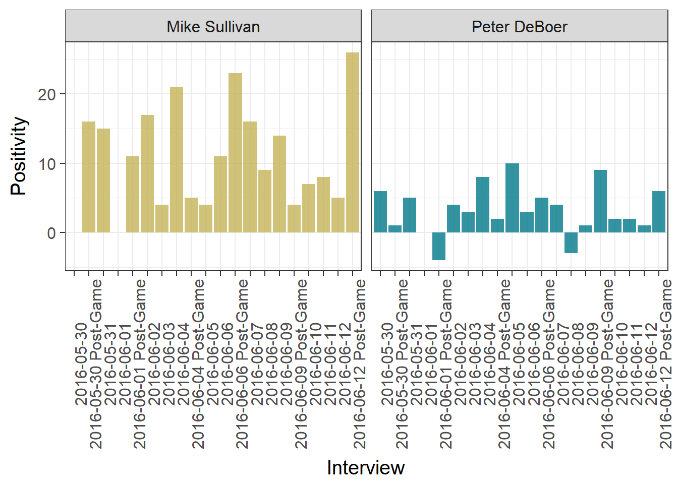

We notice the two tallest bars for each coach occur in post-game interviews for games the respective coach won, with the largest bar occurring on the post-game interview after the Penguins Cup win. The only overall negative interviews were by DeBoer, after a particularly devastating Game 2 overtime loss, and the day after a loss putting the Sharks down 3 games to 1.

A Few Things To Consider

As seen at several points in the above analyses, focusing only on individual words leads to lost context. Typically, one would also want to consider several words in a row in order to keep some context and improve the analyses. In text mining literature, we refer to these text chunks as n-grams, where n refers to the number of consecutive words to consider at once. In particular, bigrams represent chunks of two words at a time.

The tidytext package allows us to extract the bigrams from the text. We further separate the two words in each bigram and filter out those where either the first or second word is a stop word. Here are a few examples of common bigrams in the coach interviews:

## Bigrams

# Collect bigrams from text
bigrams <- coaches.text %>%
  unnest_tokens(Bigram, Text, token="ngrams", n=2) %>%
  separate(Bigram,c("Word1","Word2"),sep=" ")

# Count bigrams, show those that appear at least 5 times
bigram.counts <- bigrams %>%
  filter(!Word1 %in% stop_words$word) %>%
  filter(!Word2 %in% stop_words$word) %>%
  count(Word1,Word2,sort=T) %>%
  rename(Occurrences = n) %>%
  filter(Occurrences >= 5)

bigram.counts

## # A tibble: 15 x 3
##        Word1   Word2 Occurrences
##        <chr>   <chr>       <int>
##  1      post  season          21
##  2       san    jose          14
##  3  coaching   staff          13
##  4     power    play          12
##  5 extremely    hard          10
##  6      team     win          10
##  7      zone    time           9
##  8   scoring chances           8
##  9       top players           7
## 10   regular  season           6
## 11   stanley     cup           6
## 12  muhammad     ali           5
## 13     score   goals           5
## 14      shot   clock           5
## 15  terrific     job           5

Again, no real surprises from what someone would expect a hockey coach to be talking about, save for another reminder of Muhammad Ali’s passing.

In particular, for sentiment analysis, one needs to pay attention to negation. For example, if we run analysis on individual words, and one such word was ‘good’, we would assume this would be associated with a positive sentiment. This is obviously not the case if ‘good’ were immediately preceded by ‘not’. In the case of the coaches interviews, the following snippet shows a few instances that may have caused some issues in our previous analysis, though based on the counts, these may be negligble (indeed, if terms like ‘not afraid’ or ‘not worried’ were brought up, this may be a signal that the team is, in fact, afraid or worried).

negation.words <- c("not", "no", "never", "without")

# Find words preceded by negation words
negated.words <- bigrams %>%
  filter(Word1 %in% negation.words) %>% # First word of bigram is a negation word
  inner_join(get_sentiments("bing"), by = c(Word2 = "word")) %>% # Second word appears in sentiment data set
  count(Word1, Word2, sentiment, sort = TRUE) %>%
  ungroup()%>%
  rename(Sentiment = sentiment, Occurrences = n)

negated.words

## # A tibble: 13 x 4
##    Word1       Word2 Sentiment Occurrences
##    <chr>       <chr>     <chr>       <int>
##  1   not      enough  positive           3
##  2    no       magic  positive           2
##  3   not        like  positive           2
##  4    no       burns  negative           1
##  5    no       issue  negative           1
##  6   not      afraid  negative           1
##  7   not   available  positive           1
##  8   not complaining  negative           1
##  9   not   concerned  negative           1
## 10   not        easy  positive           1
## 11   not       ideal  positive           1
## 12   not   realistic  positive           1
## 13   not     worried  negative           1

That’s probably enough for now. I assume the extreme reserve these coaches take with regard to the media is a pretty large limitation for text analysis of their interviews, though at least we were able to see some interesting, if not largely expected results. I have some ideas for applications of these kind of techniques on other kinds of hockey-centric text data (maybe making use of Twitter…), but these will have to wait for another time!