Interactive NCAA Hockey Player Maps using ggmap, ggimage, ggiraph, and leaflet
Code for the maps can be found on Github.
Note that some of the maps on this page are static. To interact with the maps, visit the Shiny app.
Been looking at some NCAA hockey data lately. Have a few ideas kicking around, none of which are really beyond the idea stage at this point… In the meantime, since I haven’t posted anything in a while, I figured I could at least put up something fun. So here are some maps of the men’s NCAA hockey players’ hometowns, which I made using a bunch of packages in R, namely ggmap, ggimage, ggiraph and leaflet.
The ggmap package, by David Kahle and Hadley Wickham, allows the user to draw plots on top of Google Maps, plus other features such as geocoding. ggimage, by Guangchang Yu, allows a user to plot images as points. ggiraph, by David Gohel, adds interactivity to plots, which here we’ll use to display player biographical information as a tooltip. Finally, the leaflet package, by Vladimir Agafonkin et al., provides an R implementation of the Javascript Leaflet library for creating and working with interactive maps.
I’ve put together a Shiny app where you can interact with the maps from this post. Originally, I wanted to use ggmap for the plots, as I had been using that package to produce spatial visualizations for other projects. Of course, it turns out the leaflet package does all of what I wanted to do much more easily and with many additional features. I’ll talk about how to make maps using both of these packages here.
We’ll start as always by loading some handy libraries.
library(dplyr) # Really should be default
library(rvest) # Scrape scrape scrape
library(tm) # Work with strings
library(stringi) # Need 'stri_trans_general' function to standardize scraped strings
library(ggmap) # Google maps and geocoding
library(ggimage) # To plot logo icons
library(ggiraph) # Add tooltips to ggplots
library(leaflet) # Interactive maps
Gathering the data and determining hometown coordinates
As always we first need to gather the required data. For those not interested in the nuts and bolts, feel free to skip down to see the maps.
We’ll collect the biographical information for all players in NCAA D-1 men’s hockey for the 2016-2017 season from the collegehockeystats website, by looping (gasp!) through the individual team pages, scraping the biographical table for each team and binding together all the tables together at the end. Each team URL begins with http://collegehockeystats.net/1617/rosters/ and ends with a four-letter code (e.g. for Michigan, the code is “micm”). Because I am a lazy jerk, I have collected the individual URL string for each team in a separate file, which can be found on my Github.
# Table of URL codes for each team
team.urls <- read.csv("TeamCodes.csv",header=T,stringsAsFactors=F)

# Will collect tables sequentially as a list
opponent.info.list <- list()

for (i in 1:nrow(team.urls)){

  var.list <- team.urls[i,]
  opponent.info.list[[i]] <- collect.player.info(var.list)

  Sys.sleep(3) # So that collegehockeystats doesn't get fussy...

}

players <- bind_rows(opponent.info.list) # Merge all tables together into onehead(players)## Number Name Class Position Hometown
## 1 2 Kyle Mackey JR D Derby, New York
## 2 3 Johnny Hrabovsky SR D Humelstown, Pennsylvania
## 3 4 Phil Boje JR D Shoreview, Minnesota
## 4 6 Mathew Buchill FR D Marshfield, Massachusetts
## 5 7 Matt Koch SO D Hastings, Minnesota
## 6 9 Trevor Stone FR F Pleasant Plains, Illinois
## Team Simple.Hometown
## 1 Air Force derby new york
## 2 Air Force humelstown pennsylvania
## 3 Air Force shoreview minnesota
## 4 Air Force marshfield massachusetts
## 5 Air Force hastings minnesota
## 6 Air Force pleasant plains illinois
## Label
## 1 Air Force: 02 Kyle Mackey - Derby, New York (JR-D)
## 2 Air Force: 03 Johnny Hrabovsky - Humelstown, Pennsylvania (SR-D)
## 3 Air Force: 04 Phil Boje - Shoreview, Minnesota (JR-D)
## 4 Air Force: 06 Mathew Buchill - Marshfield, Massachusetts (FR-D)
## 5 Air Force: 07 Matt Koch - Hastings, Minnesota (SO-D)
## 6 Air Force: 09 Trevor Stone - Pleasant Plains, Illinois (FR-F)The code snippet above calls collect.player.info, written below. This function, in addition to scraping the bio, converts the strings into a useful format for later use. In particular, the extract.hometown function separates and discards the previous Junior team information from the biography string (e.g. for, say, Michigan, the “Hometown/Last Team column” reads “Mississauga, Ontario / Janesville Jets (NAHL)”). The simplify.hometown function makes the hometown more easily readible by ggmap functions, which will come in handy later for geocoding. More details can be found in the comments below.
# Some players have their NHL draft team in parantheses next to their name
remove.drafted.team <- function(name) {

  name.tokens <- unlist(strsplit(name," ")) # Split name into tokens

  k <- length(name.tokens) # Get number of tokens

  if (grepl(x=name.tokens[k],pattern="\\(")){ # If the last token begins with a parantheses...
    name.tokens <- name.tokens[-k] # ...toss it out
  }

  return(paste(name.tokens,collapse= " ")) # Paste name string back together

}

# Hometown string also has previous team affiliation; get rid of that
extract.hometown <- function(hometown.string){

  tokens <- unlist(strsplit(hometown.string,"/")) # Split string into tokens

  hometown <- trimws(tokens[1]) # Extract the first token and trim the whitespace on each end

  return(hometown)

}

# For use with "geocode" function, simplify the hometown string
simplify.hometown <- function(hometown.string){

  hometown <- removePunctuation(tolower(hometown.string)) # Remove punctuation and put into all lower case

  return(hometown)

}

# Puts together a label for each player to assign as tooltips for maps
assign.label <- function(team,number,name,class,position,hometown){

  if (number < 10){ # Force number to have 2 digits
    number.label<-paste0("0",number)
  } else {
    number.label<-as.character(number)
  }

  # Remove single-quotes "'"; causes problems with leaflet
  hometown.label <- gsub(hometown,pattern="'",replacement="")

  # Paste info together in nice format
  return(paste0(team,": ",number.label," ",name," - ",hometown," (",class,"-", position,")"))
}

# Scrape player table for each team
collect.player.info <- function(var.list) {

  # Get URL
  team <- var.list$Team[1]
  code <- var.list$Code[1]

  url <- paste0("http://collegehockeystats.net/1617/rosters/",code) # For year 2016-2017

  # Scrape table
  player.info <-  url %>% read_html %>%
    html_nodes('.rostable') %>% # This is the table we need
    html_table(header=T, fill=T) %>%
    data.frame(stringsAsFactors = F)

  player.info <- player.info[,1:9]

  # Add column names
  names(player.info) <- c("Number","Name","Class","Position","Height","Weight","Shoots","YOB","Hometown")

  # Convert strings to all ASCII; random characters screw with ggmap and leaflet
  player.info$Name <- stri_trans_general(player.info$Name,"Latin-ASCII")
  player.info$Hometown <- stri_trans_general(player.info$Hometown,"Latin-ASCII")

  # Assemble clean table
  player.info.clean <- player.info %>%
    rowwise() %>%
    select(Number,Name,Class,Position,Hometown) %>%
    mutate(Team = team,
           Number = as.numeric(gsub(Number,pattern="#",replacement = "")),
           # Weird gsub below gets rid of weird spaces (may not be necessary?)
           Name = remove.drafted.team(gsub("[^\\x{00}-\\x{7f}]", " ", Name, perl = TRUE)),
           Class = gsub("[^\\x{00}-\\x{7f}]", " ", Class, perl = TRUE),
           Hometown = extract.hometown(Hometown),
           Simple.Hometown = simplify.hometown(Hometown),
           Label = assign.label(Team,Number,Name,Class,Position,Hometown))

  print(paste0("Completed Scraping for ", team)) # Track progress

  return(player.info.clean)
}
We have the player bios with the hometowns extracted into their own column. Now we need to get the geographical coordinates for each hometown. We’ll do this in a second pass of another loop (another gasp!), using the geocode function from the ggmap package, which returns a bunch of information related to a search of the hometown. Here we need just the latitude and longitude coordinates of the hometown for plotting.
Despite having cleaned out most of the anomalies from the hometown strings, my first run of geocode still crashed a number of times. It seems a few weird characters still made it through. Taking a look at all hometowns with non-alphanumeric characters…
# Still a few weird characters in the data set. Let's see which are causing problems
troublesome.hometowns <- players %>%
  rowwise() %>%
  filter(grepl('[^[:alnum:] ]',Simple.Hometown))

head(troublesome.hometowns %>% select(Team,Name,Simple.Hometown)) ## # A tibble: 6 x 3
## Team Name Simple.Hometown
## <chr> <chr> <chr>
## 1 Alabama-Huntsville Carmine Guerriero montr<U+FFFD>al quebec
## 2 Alaska-Anchorage Nicolas Erb-Ekholm malm<U+FFFD> sweden
## 3 American International Zackarias Skog g<U+FFFD>teborg sweden
## 4 American International Dominik Florian vla<U+009A>im czech republic
## 5 Arizona State Jakob Stridsberg j<U+FFFD>nkoping sweden
## 6 Bemidji State Dylan McCrory kirkland qu<U+FFFD>becThe biggest offenders appear to be french accented characters in Quebecois cities, and other accents on some European cities. Again, lazy jerk, I ended up just manually fixing these, at which point geocode runs without issue. For those (few) players with hometowns where no coordinates are returned, they get tossed out of the dataset :(
# There are a few players with no hometown, so let's toss them out
players <- players %>%
  filter(!is.na(Simple.Hometown))

# Append sequentially the results of the 'geocode' function
# Extract latitude and longitude of the hometown
for(i in 1:nrow(players)) {

  result <- geocode(players$Simple.Hometown[i], output = "latlona", source = "google") # Get coordinates

  # Extract coordinates
  players$Lon[i] <- as.numeric(result[1])
  players$Lat[i] <- as.numeric(result[2])
}

# Toss out players that 'geocode' couldn't find
players <- players %>%
filter(!is.na(Lat),!is.na(Lon))head(players)## Number Name Class Position Hometown
## 1 2 Kyle Mackey JR D Derby, New York
## 2 3 Johnny Hrabovsky SR D Humelstown, Pennsylvania
## 3 4 Phil Boje JR D Shoreview, Minnesota
## 4 6 Mathew Buchill FR D Marshfield, Massachusetts
## 5 7 Matt Koch SO D Hastings, Minnesota
## 6 9 Trevor Stone FR F Pleasant Plains, Illinois
## Team Simple.Hometown
## 1 Air Force derby new york
## 2 Air Force humelstown pennsylvania
## 3 Air Force shoreview minnesota
## 4 Air Force marshfield massachusetts
## 5 Air Force hastings minnesota
## 6 Air Force pleasant plains illinois
## Label
## 1 Air Force: 02 Kyle Mackey - Derby, New York (JR-D)
## 2 Air Force: 03 Johnny Hrabovsky - Humelstown, Pennsylvania (SR-D)
## 3 Air Force: 04 Phil Boje - Shoreview, Minnesota (JR-D)
## 4 Air Force: 06 Mathew Buchill - Marshfield, Massachusetts (FR-D)
## 5 Air Force: 07 Matt Koch - Hastings, Minnesota (SO-D)
## 6 Air Force: 09 Trevor Stone - Pleasant Plains, Illinois (FR-F)
## Lon Lat
## 1 -78.97973 42.68645
## 2 -76.70830 40.26537
## 3 -93.14717 45.07913
## 4 -70.70559 42.09175
## 5 -92.85137 44.74433
## 6 -89.92122 39.87283I’ll be adding the team logos to the plots as markers for our maps. For the purposes of this post, all you need to know is that the logo.images file has three columns: Team with the team name, Color with the hexcode of the main color for each team, and Image for the location of the image file for the team’s logo. To make examples more reproducible, I’ll show how to code the maps both with and without logo markers.
all.teams <- unique(logo.images$Team)
player.colors <- logo.images$Color
names(player.colors) <- all.teamsset.seed(90707)
players <- players %>%
left_join(logo.images,by="Team") %>%
rowwise() %>%
mutate(Lon = Lon + runif(1,min=-0.025,max=0.025), # Add some jitter to coordinates
Lat = Lat + runif(1,min=-0.025,max=0.025)) # (so that players in one city aren't stacked on top of one another)Using ggmap
A ggmap is initiated using get_map, which returns a map of a specified area. This is then fed into the ggmap function. Here, we use the geom_image function from the ggimage package to plot the logos as markers, using the latitude and longitude values found earlier.
area <- "Ann Arbor, Michigan"
zoom <- 4

center <- geocode(area, output = "latlona", source = "google")
center.lon <- as.numeric(center[1])
center.lat <- as.numeric(center[2])
# With logos
plot <- ggmap(get_map(area, zoom=zoom)) + # Load map of area
geom_image(aes(x=Lon, y=Lat, image=Image), data=players, size=0.04, alpha=0.8) + # Add logos
ggplot2::annotate("text", x=center.lon, y=center.lat,
col="red", label="@mathieubray", alpha=0.2, cex=30, fontface="bold", angle=30) + # Watermark
geom_point_interactive(aes(x=Lon, y=Lat, tooltip=Label),
size=15, alpha=0.01, data=players) + # Add interactive points underneath logos
theme(axis.title.x=element_blank(), axis.text.x=element_blank(), axis.ticks.x=element_blank(), # Remove axes
axis.title.y=element_blank(), axis.text.y=element_blank(), axis.ticks.y=element_blank())
ggiraph(code={print(plot)}, width=1, width_svg=20, height_svg=16) # Interactive plot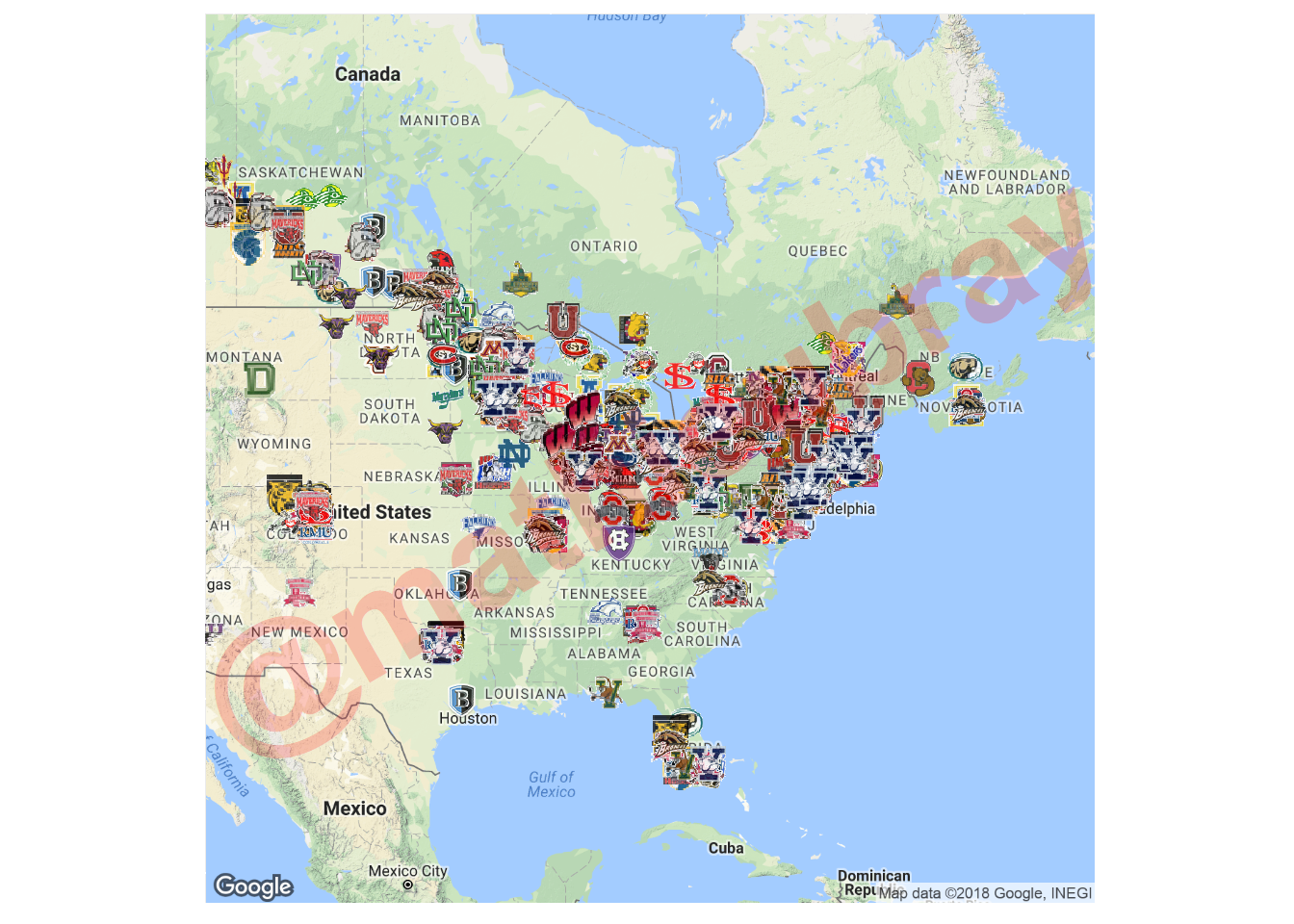
In supported environemnts, to display the player information as a tooltip, we use the geom_point_interactive function from the ggiraph package (essentially, this places large transparent points underneath each logo which will interact with mouse movement). The final plot is rendered using the ggiraph function.
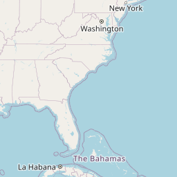
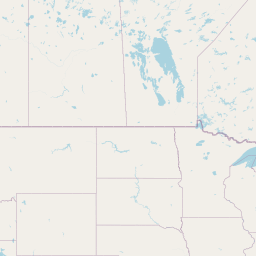
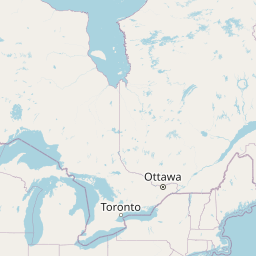
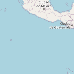
This first plot is quite busy, showing the entire set of players from the 2016-2017 season. We can see a few players from non-traditional hockey places outside of the US-Canada border, such as Montana, New Mexico, and Northwest Florida (Bentley in particular seems to draw interest from some non-traditional areas, Houston and Oklahoma). Suppose we wanted to focus on, for example, just Big Ten teams, in some area with high activity, say Detroit…
# With logos

plot <- ggmap(get_map(area, zoom=zoom)) + # Load map of area
  geom_image(aes(x=Lon, y=Lat, image=Image), data = big.ten, size=0.04, alpha=0.8) + # Add logos
  ggplot2::annotate("text", x=center.lon, y=center.lat,
                    col="red", label="@mathieubray", alpha=0.2, cex=30, fontface="bold", angle=30) + # Watermark
  geom_point_interactive(aes(x=Lon, y=Lat, tooltip=Label),
                         size=15, alpha=0.01, data=players) + # Add interactive points underneath logos
  theme(axis.title.x=element_blank(), axis.text.x=element_blank(), axis.ticks.x=element_blank(), # Remove axes
        axis.title.y=element_blank(), axis.text.y=element_blank(), axis.ticks.y=element_blank())

ggiraph(code={print(plot)}, width=1, width_svg=20, height_svg=16) # Interactive plot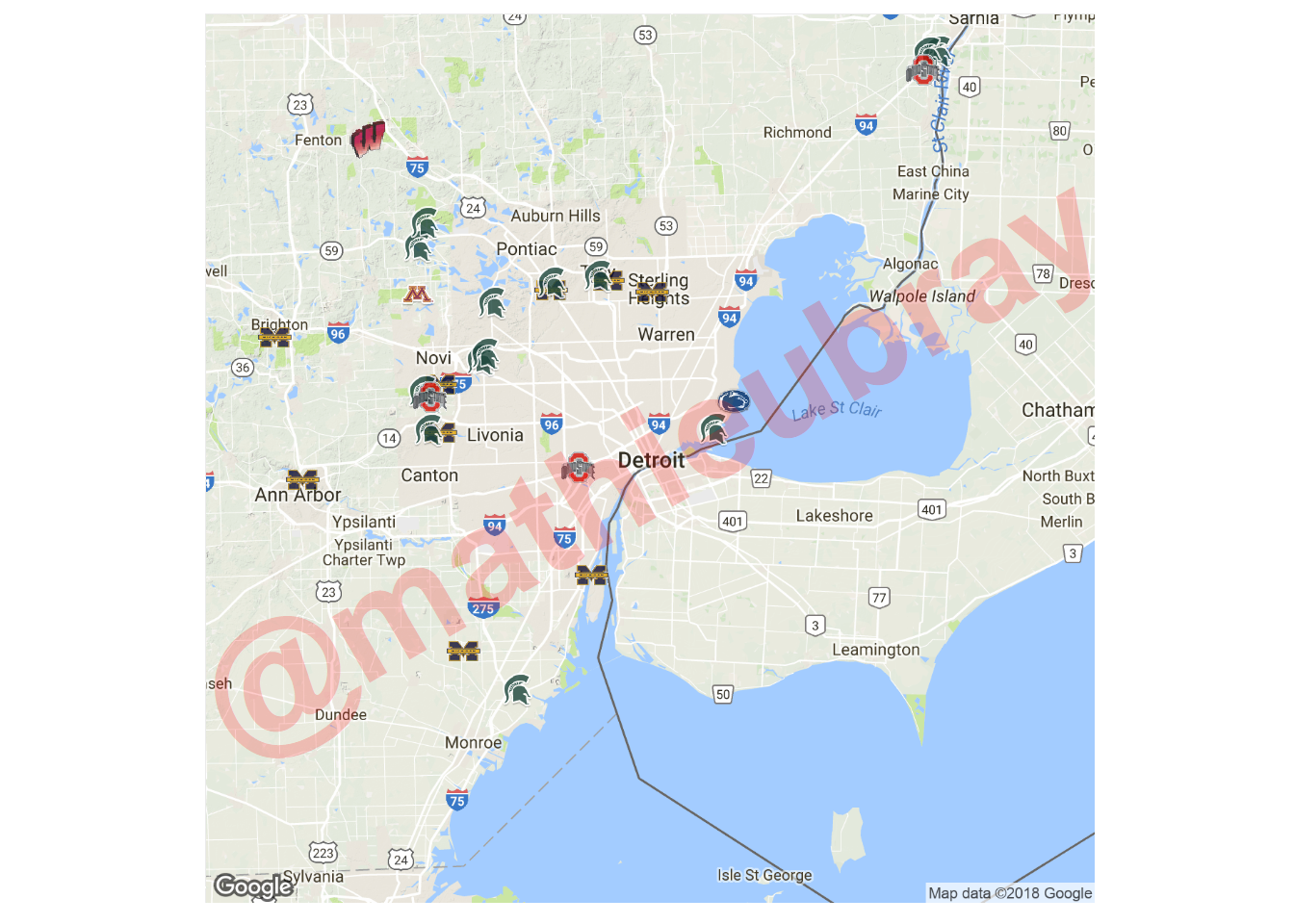
To plot maps without logos, we color the points generated by geom_point_interactive with a different color for each Team, instead of using geom_image. Here, I map each team to the Color value from the logo.images data set using scale_fill_manual, but colors will be automatically added as well if that line of code is removed.
# Without logos

plot <- ggmap(get_map(area, zoom=zoom)) + # Load map of area
  ggplot2::annotate("text", x=center.lon, y=center.lat,
                    col="red", label="@mathieubray", alpha=0.2, cex=30, fontface="bold", angle=30) + # Watermark
  geom_point_interactive(aes(x=Lon, y=Lat, tooltip=Label, fill=Team),
                         pch=21, color="black", size=10, alpha=0.5, data=players) + # Add interactive points
  scale_fill_manual(values=player.colors) + # Change color of points
  guides(fill=guide_legend(override.aes=list(alpha=1))) + # Format legend and remove axes
  theme(axis.title.x=element_blank(), axis.text.x=element_blank(), axis.ticks.x=element_blank(),
        axis.title.y=element_blank(), axis.text.y=element_blank(), axis.ticks.y=element_blank(),
        legend.position="bottom", legend.title = element_blank(), legend.text=element_text(size=20))
# Without logos
plot <- ggmap(get_map(area, zoom=zoom)) + # Load map of area
ggplot2::annotate("text", x=center.lon, y=center.lat,
col="red", label="@mathieubray", alpha=0.2, cex=30, fontface="bold", angle=30) + # Watermark
geom_point_interactive(aes(x=Lon, y=Lat, tooltip=Label, fill=Team),
pch=21, color="black", size=10, alpha=0.5, data=players) + # Add interactive points
scale_fill_manual(values=player.colors) + # Change color of points
guides(fill=guide_legend(override.aes=list(alpha=1))) + # Format legend and remove axes
theme(axis.title.x=element_blank(), axis.text.x=element_blank(), axis.ticks.x=element_blank(),
axis.title.y=element_blank(), axis.text.y=element_blank(), axis.ticks.y=element_blank(),
legend.position="bottom", legend.title = element_blank(), legend.text=element_text(size=20))
ggiraph(code={print(plot)}, width=1, width_svg=24, height_svg=20) # Interactive plot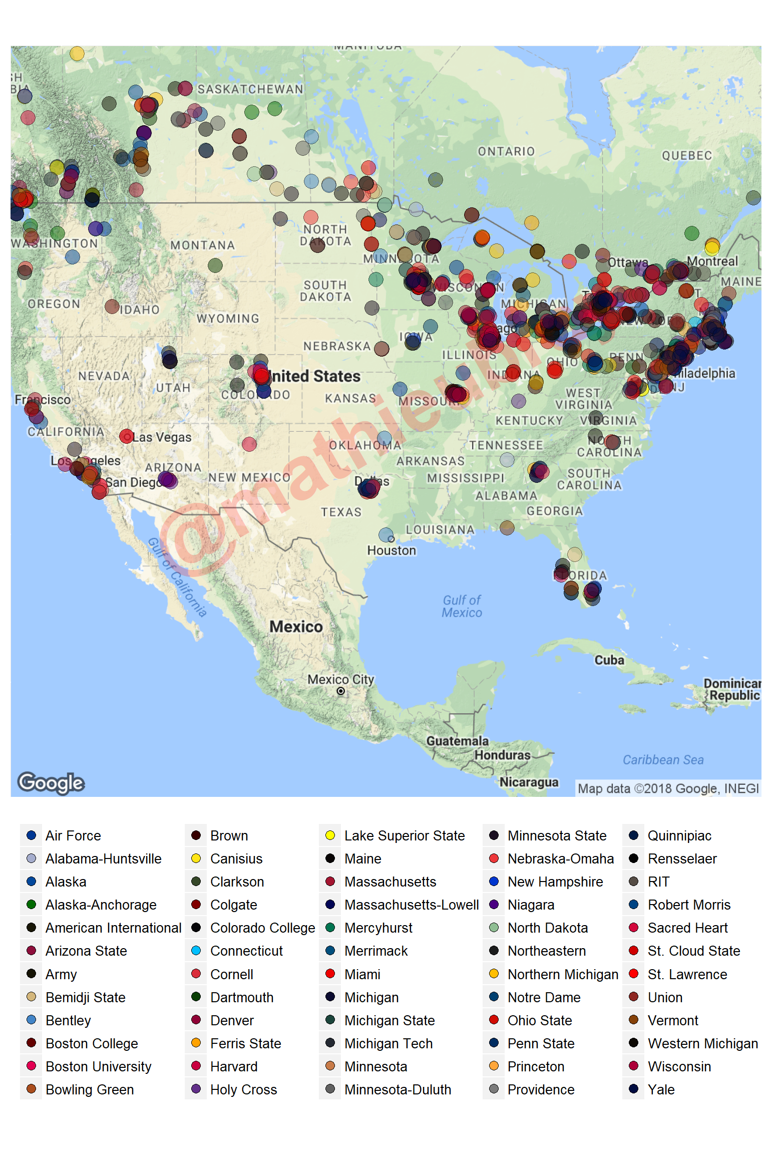
Using leaflet
While the packages above come together to make a nifty map, they are quite rigid, with only static images shown, and the area and zoom needing to be reset manually anytime we want to check out a new location. Fortunately, leaflet has a suite of functions for much simpler plotting, and allows one to zoom and change location automatically in supported environemnts. Leaflet is used by a number of leading web companies, including Craigslist notably…
We add the logo images indivdually using makeIcon, and assemble them in an iconList, which will be supplied to the leaflet plotting function. Note that I had to code each team’s icon individually because I couldn’t figure out how to make iconList work with the usual apply-family functions (any suggestions?). The screenshot of the full map is shown below.
# Plot map using package 'leaflet'
# With Logos

get.file <- function(team){ # Extract image file

  image <- logo.images %>%
    filter(Team == team) %>%
    .$Image %>%
    unique

  return(image)
}

logos <- iconList( # Is there a better way to do this?

  "Air Force" = makeIcon(get.file("Air Force")),
  "Alabama-Huntsville" = makeIcon(get.file("Alabama-Huntsville")),
  ...
  "Yale" = makeIcon(get.file("Yale"))
)leaflet(data = players, options=leafletOptions(worldCopyJump=T)) %>%
addTiles() %>% # Map
addControl("<b><p style='font-family:arial; font-size:36px; opacity:0.2; '><a href='https://twitter.com/mathieubray' style='color:red; text-decoration:none; '>@mathieubray</a></p>",
position="bottomleft") %>% # Watermark
addMarkers(~Lon, ~Lat,
label=~Label,
icon=~logos[Team],
options = markerOptions(opacity=0.8),
labelOptions=labelOptions(offset=c(20,0))) %>%
setView(lng=center.lon, lat=center.lat, zoom=zoom) # Set default view


Again, while interesting, the initial view above is quite busy (though if you were, say, in the Shiny app, you could zoom in and out in this case). To further declutter the view, the leaflet package has functionality to cluster nearby data points. A simple line of code gets us what we want.
leaflet(data = players, options=leafletOptions(worldCopyJump=T)) %>%
  addTiles() %>% # Map
  addControl("<b><p style='font-family:arial; font-size:36px; opacity:0.2; '><a href='https://twitter.com/mathieubray' style='color:red; text-decoration:none; '>@mathieubray</a></p>",
             position="bottomleft") %>% # Watermark
  addMarkers(~Lon, ~Lat,
             label=~Label,
             icon=~logos[Team],
             options = markerOptions(opacity=0.8),
             labelOptions=labelOptions(offset=c(20,0)),
             clusterOptions=markerClusterOptions()) %>% # Group nearby points into clusters
setView(lng=center.lon, lat=center.lat, zoom=zoom) # Set default viewTo suppress logos, the code snippet below creates a mapping for each player to an awesomeIcon with a distinct color for each team. These are included in the plot using the addAwesomeMarkers function.
# Without Logos

logo.color <- function(logos){

  lapply(logos$Team, function(team) { # Extract color

    color <- logos %>%
      filter(Team == team) %>%
      .$Color %>%
      unique

    return(color)
  })

}

icons <- awesomeIcons( # Assign color to each icon based on team

  icon = 'record',
  iconColor = logo.color(players),
  library = 'ion',
  markerColor = 'white'

)

leaflet(data=players, options=leafletOptions(worldCopyJump=T)) %>%
  addTiles() %>% # Map
  addControl("<b><p style='font-family:arial; font-size:36px; opacity:0.2; '><a href='https://twitter.com/mathieubray' style='color:red; text-decoration:none; '>@mathieubray</a></p>",
             position="bottomleft") %>% # Watermark
  addAwesomeMarkers(~Lon, ~Lat,
                    label = ~as.character(Label),
                    icon = icons,
                    clusterOptions=markerClusterOptions()) %>%
setView(lng=center.lon, lat=center.lat, zoom=zoom)Fun, fun stuff. Again, check out the Shiny app, where you can interact with the maps generated by both ggmap and leaflet. Note that ggimage and Shiny don’t seem to play very well together, so the ggmap plots in the app don’t have logos (for now at least). Anyway, keep well, and see you next time!