An Introduction to Kidney Paired Donation, with ompr and ggraph
Code for this worked example can be found on Github.
While most of my work posted here over the past year has been inspired by hockey statistics, the majority of my time is spent doing actual work on a much more important problem.
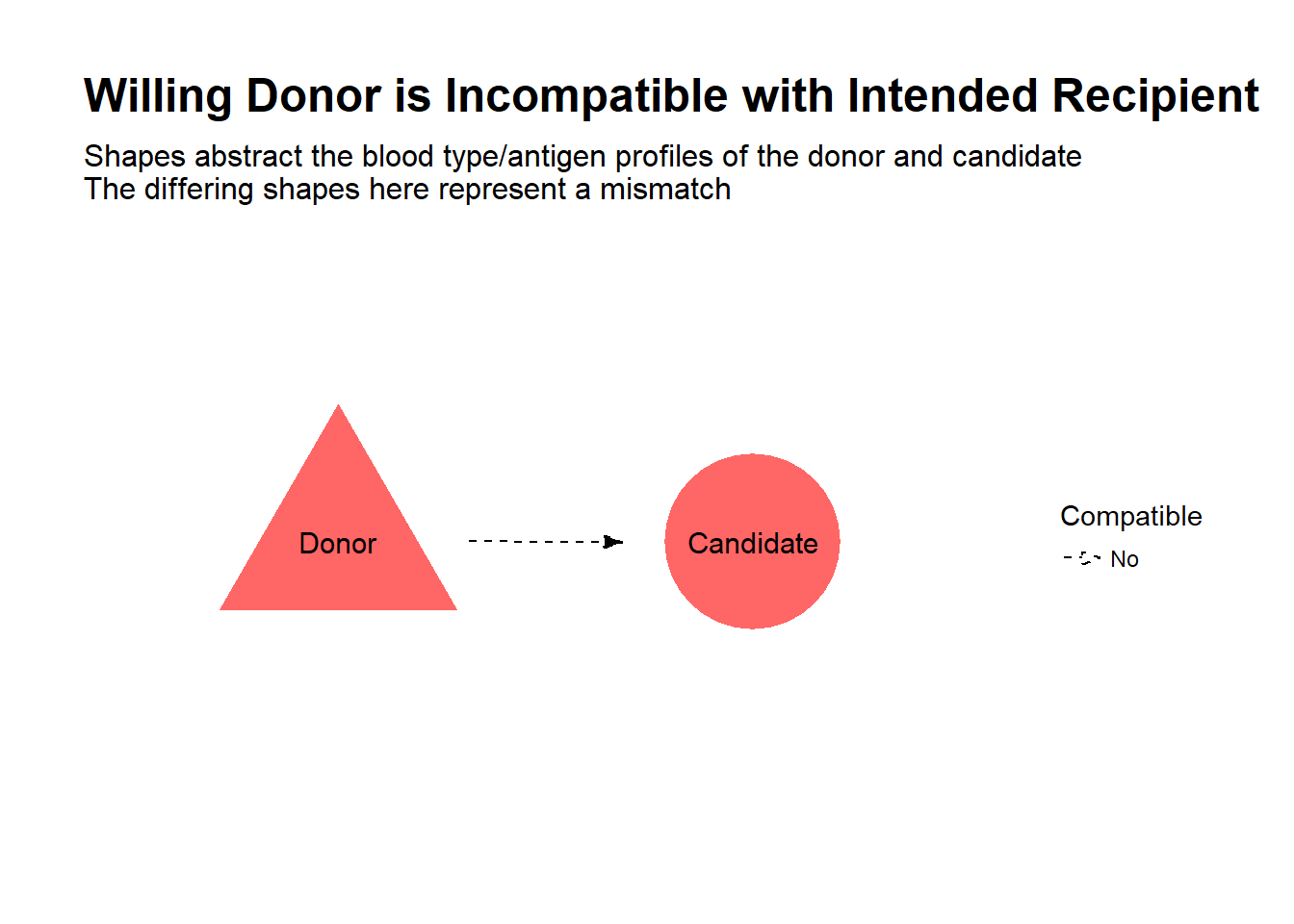
Let’s say you know someone in need of a kidney transplant, and after careful reflection on the risks, you are willing to donate one of your kidneys to your friend. This is one option for kidney transplant candidates, to avoid potentially long waits on the deceased donor list and improve their quality of life compared to continued dialysis. However, in your case, we find that the transplant would be incompatible, due to a mismatch of blood types or antigen profiles between you and your friend, and therefore cannot proceed.
Is all hope lost? Well, suppose there was another dialysis patient in the same boat, also with a willing but incompatible donor. Now, suppose it turns out you are compatible with the other patient, and her donor is compatible with your friend. By simply swapping donors, both patients receive a transplant!
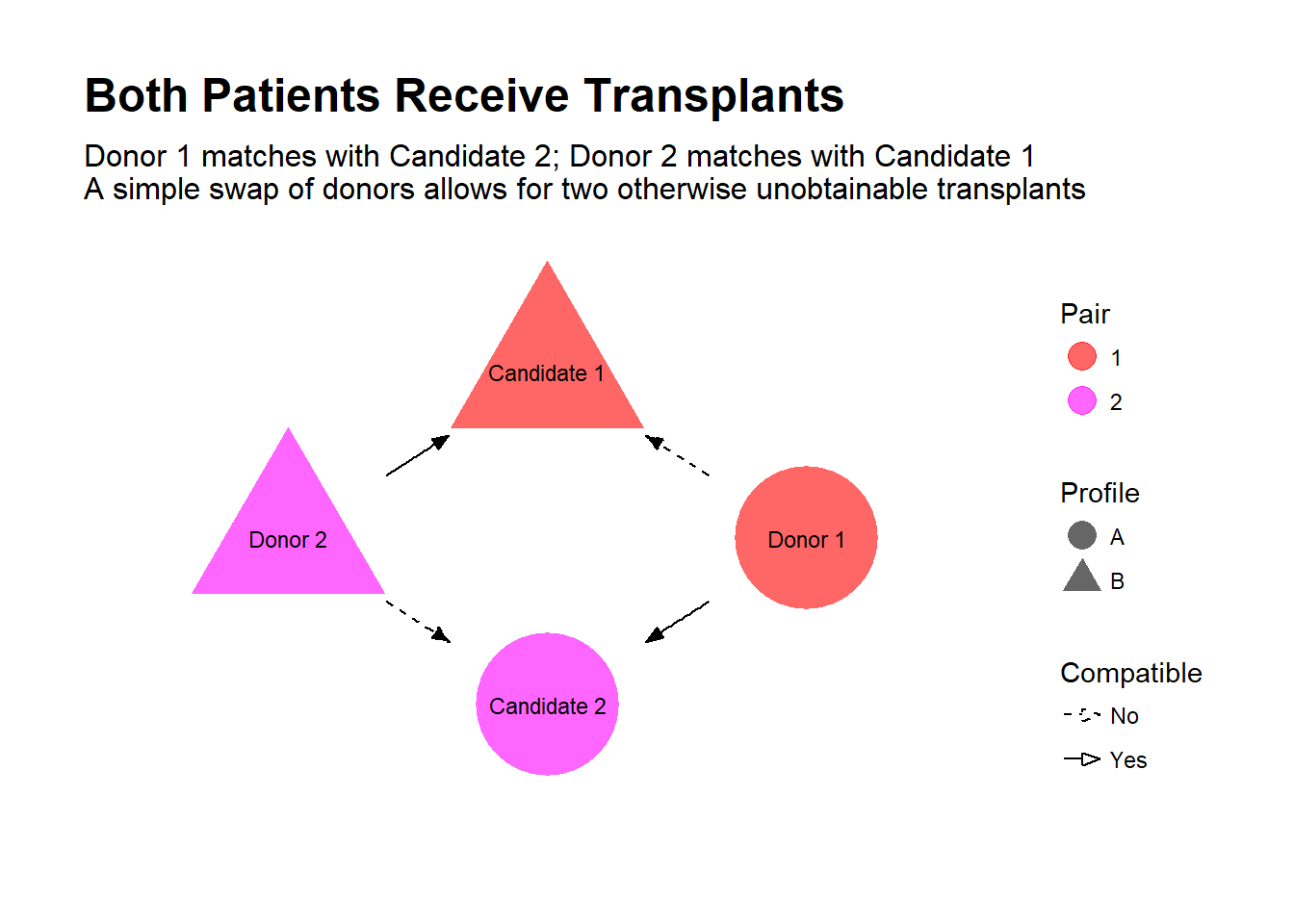
This is the idea behind kidney-paired donation (KPD), where incompatible donor-candidate pairs are pooled in an effort to find exchanges that allow for new transplant opportunities. Some transplant centers in the U.S. that run their own KPD programs, and partnerships exist between transplant centers, such as the Alliance for Paired Donation.
The main question is, which exchanges should be selected for transplantation at any given time? In its simplest form, the goal is to achieve the highest number of transplants possible.
In the rest of this post, I’ll lay out the mathematical formulation of KPD and work through an example, while also demonstrating some R packages I’ve been using lately.
*Selected references for this topic: Roth et al, 2004; Roth et al, 2005; Segev et al, 2005; Gentry et al, 2011; Li et al, 2014
A mathematical model for KPD
A KPD pool can be abstracted as a network/graph, where nodes represent pairs (i.e. a transplant candidate together with her donor), and directed edges are formed between two nodes when the donor from the first node is compatible with the transplant candidate in the second node.
How are transplants obtained? Well, each donor has one kidney to give and each candidate need only receive one kidney. We require that for every donor who donates a kidney, that their paired candidate receive a kidney in return. A sequence of donations must end with the donor of the final pair donating to the candidate from the first pair. Thus, exchanges are closed cycles in our graph.
KPD programs can also include candidates who join with several incompatible donors, compatible pairs, and altruistic donors (who start chains of transplants, with no requirement that the final donor return the favor to any particular candidate). All of these add their own subtle nuances to the KPD problem, but for the purposes of this demonstration, we will restrict ourselves to the case where each candidate joins the program with a single incompatible donor.
What exchanges should be pursued for transplantation? KPD can be seen as an example of a cycle packing problem, where the goal is to find the disjoint set of cycles such that the combined weight of their constituent edges is maximized. In the KPD problem, we typically want the solution that admits the maximum number of transplants, and so each edge is effectively given a weight of 1. In general, this problem is NP-hard (unless the cycle size is restricted to 2, in which case the problem reduces to a maximum weighted matching problem). However, with a manageable pool size, a restricted maximum cycle size and a reasonably sparse graph, the processing power will generally overcome the theoretical burden of the solving algorithms.
Solving the KPD problem using ompr
We will generate an example KPD pool and determine the best set of exchanges to pursue. We will use the ompr package, by Dirk Schumacher to solve the integer programming problem. I will also demonstrate the ggraph package, for plotting networks, by Thomas Lin Pedersen.
First, let’s load our handy libraries.
library(dplyr) # Take that, base R
library(purrr) # 'map' functions
library(igraph) # R graph framework
library(ggplot2) # For plotting
library(ggraph) # Plotting graphs
library(data.table) # 'rbindlist' to combine list of data frames into one data frame

library(ompr) # Mixed integer programming
library(ompr.roi)
library(ROI) # R optimization interface
library(ROI.plugin.glpk) # Will use solver 'glpk'
We start with a KPD pool with 20 pairs, where every possible match between two pairs has a 0.1 probability of forming an edge. This is an example of an Erdo-Renyi random graph, which will suffice for our demonstration (in reality, since potential matches are evaluated based on blood type and antigen profiles, some nodes are inherently more likely to either be matched with or match to other pairs). We use the sample_gnp function from the igraph package to accomplish this.
We use the ggraph package to visualize the KPD pool. This package allows for easy graph plotting of igraph objects, in the same vein as ggplot2. Edges are added to the plot using the geom_edge_* functions (here we simply use geom_edge_link to draw arrows, but other types of edges are possible). Similarly, nodes can be drawn using geom_node_* functions. Here we use geom_node_point to draw the nodes and geom_node_text to add labels. More information can be found here.
set.seed(901) # Arbitrary seed, seemed to generate a decent network for this demo

number_of_nodes  <- 20

kpd <- sample_gnp(number_of_nodes, 0.1, directed=TRUE) # Here we generate our KPD as a Erdos-Renyi random graph

# Plot graph
ggraph(kpd,layout='linear',circular=TRUE) +
  geom_edge_link(start_cap=circle(5,"mm"),
                     end_cap=circle(5,"mm"),
                 show.legend=FALSE,
                 arrow=arrow(angle=20,
                             length=unit(0.1,"inches"),
                             type="closed")) +
  geom_node_point(size=12,color="red",alpha=0.6) +
  geom_node_text(aes(label=1:20),size=5,color="black") +
  theme_graph()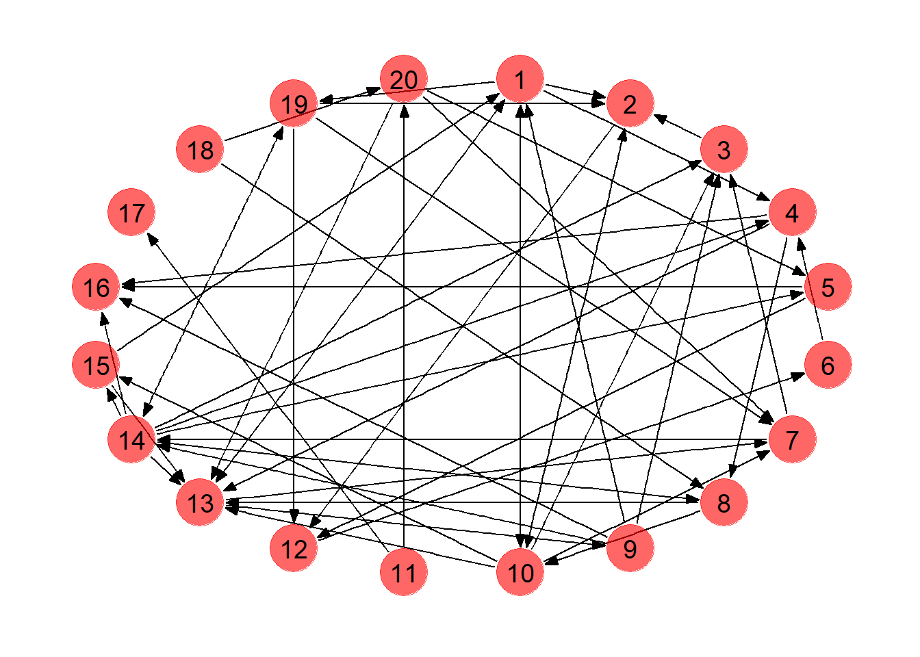
We collect the edges of the graph in a separate data frame which will come in handy later. You can confirm the edges shown below appear in the KPD network above.
# Retrieve edges in the network
edges <- kpd %>% get.edgelist %>% data.frame

edges %>% rename(from=X1,to=X2) %>% head## from to
## 1 9 1
## 2 10 1
## 3 13 1
## 4 15 1
## 5 1 2
## 6 3 2An obvious first step would be to find a set of possible exchanges in the pool. For this we need a function that extracts all the cycles from our network. Since I couldn’t seem to find an existing function to extract cycles (at least not to my knowledge? igraph didn’t have what I was looking for…), I ended up writing my own. You can check out the techincal details of the get_cycles function at the end of this post (or click here).
The list of cycles, as well as the number of transplants each cycle admits, is shown below.
# Collect all the cycles in the network

cycle_size <- 3

cycles <- get_cycles(number_of_nodes, edges, cycle_size)
number_of_cycles <- length(cycles)


# Assign a label to each cycle
cycle_strings <- map_chr(cycles, function(x){ paste(x, collapse="-")})

# Collect separately the size of each of the cycles in the network
transplants <- purrr::map_int(cycles,length)


data.frame(cycle_strings=cycle_strings, transplants=transplants)## cycle_strings transplants
## 1 1-2-10 3
## 2 1-4-13 3
## 3 1-10 2
## 4 1-10-13 3
## 5 1-10-15 3
## 6 1-13 2
## 7 1-13-9 3
## 8 2-10 2
## 9 2-10-3 3
## 10 7-14-13 3
## 11 7-14-19 3
## 12 9-14-13 3
## 13 14-19 2Let’s highlight these nodes and edges in our plot. We first need to extract the edges involved in each cycle. The get_cycle_edges function collects the edges involved in each cycle and combines them into a handy data frame.
# For a vector representing a cycle, build data frame of the edges
get_cycle_edges <- function(cycle_node_list){

  edge_list <- data.frame(X1=numeric(), X2=numeric())

  cycle_length <- length(cycle_node_list)

  # Caution: FOR loop :( :( :(
  for(i in 1:(cycle_length - 1)){
    edge_list <- rbind(edge_list, data.frame(X1 = cycle_node_list[i], X2 = cycle_node_list[i+1]))
  }

  edge_list <- rbind(edge_list, data.frame(X1 = cycle_node_list[cycle_length], X2 = cycle_node_list[1]))
}
For each node and edge in the original pool, we tag whether it appears in a cycle or not, then plot the graph with manually assigned node colors, edge colors, widths and line types.
# Get all edges that appear in cycles
cycle_edges <- map(cycles, get_cycle_edges) %>%
  rbindlist %>%
  unique %>%
  as_tibble %>%
  mutate(in.cycle = TRUE)

# Mark each edge whether it appears in a cycle or not
edges_enhanced <- edges %>%
  left_join(cycle_edges,by=c("X1","X2")) %>%
  mutate(in.cycle = !is.na(in.cycle))

E(kpd)$Cycle <- edges_enhanced$in.cycle # Assign property to edge

edges_enhanced %>% rename(from=X1,to=X2) %>% head## from to in.cycle
## 1 9 1 TRUE
## 2 10 1 TRUE
## 3 13 1 TRUE
## 4 15 1 TRUE
## 5 1 2 TRUE
## 6 3 2 TRUE# Get all nodes that appear in cycles
cycle_nodes <- cycles %>% unlist %>% unique %>% sort
# Mark each node whether it appears in a cycle or not
node_in_cycle <- 1:number_of_nodes %in% cycle_nodes
V(kpd)$Cycle <- node_in_cycle # Assign property to node# Plot network with nodes and edges in cycles highlighted
ggraph(kpd, layout = 'circle') +
geom_edge_link(aes(edge_colour=Cycle,
edge_width=Cycle,
edge_linetype=Cycle),
start_cap=circle(5,"mm"),
end_cap=circle(5,"mm"),
arrow=arrow(angle=20,
length=unit(0.1,"inches"),
type="closed")) +
geom_node_point(aes(color=Cycle),size=12,alpha=0.6,show.legend=F) +
geom_node_text(aes(label=1:20),size=5,color="black") +
scale_color_manual(values=c("red","magenta")) +
scale_edge_color_manual(values=c("black","magenta")) +
scale_edge_width_manual(values=c(0.5,1)) +
scale_edge_linetype_manual(values=c("dotted","solid")) +
theme_graph()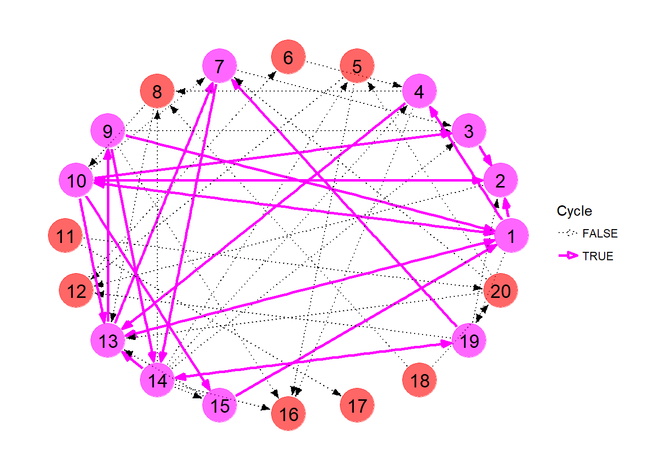
So which exchanges should we pursue? It’s kind of difficult to decide just looking at the picture. Even with the list of cycles above, the best course of action is not readily obvious.
Again, we’re looking for the set of disjoint cycles that maximizes the number of transplants among the selected exchanges. The ompr package comes in handy here. It uses a very simple syntax in order to build a solver for mixed integer problems, like the KPD problem, on top of the R Optimization Interface (ROI). The main idea is to abstract our problem, initialized using MIPModel, with variables (add_variable), establish an objective (set_objective), add constraints (add_constraint), and then solve (solve_model). We use the free glpk solver here, which is passed as an argument to the solve_model function. The solution can then be extracted into a data frame using get_solution.
We describe here the problem in such a way that we can solve it using ompr (this is a slightly different formulation than is common in the literature). Let \(C\) be the number of cycles and \(N\) be the number of nodes. Let \(U_i\) represent here the utility of the cycle. In our case, this is simply the number of transplants the cycle admits. In general, a cycle can be assigned any value of \(U_i\), reflecting certain clinical factors for example, and maximization will be effectively in terms of that utility.
Let \(Y_i \in \{0,1\}\) designate whether cycle \(i\) should be pursued (1) or not (0). Similarly, let \(X_{ij} \in \{0,1\}\) correspond to the status of node \(j\) with respect to cycle \(i\). Obviously, the status of node \(j\) is tied to the statuses of the cycles that contain it. In other words, if cycle \(i\) is chosen (i.e. \(Y_i = 1\)), and node \(j\) is part of cycle \(i\), node \(j\) is therefore chosen (i.e. \(X_{ij} = 1\)). So node \(j\) is part of cycle \(i \Rightarrow X_{ij} = Y_i\), \(i \in \{1,...,C\}, j \in \{1,...,N\}\). Obviously, a node can only appear in the solution once. So for each node \(j\), we want that \(\sum_{i}X_{ij} \leq 1\).
The optimization problem is thus summarized as follows:
\[\max_{\{Y_i\}} \sum_i Y_iU_i \\ st. \sum_{i}X_{ij} \leq 1, j \in \{1,...,N\}\\ \ X_{ij} = Y_i \ I(\mbox{Node } j \mbox{ is part of Cycle } i), i \in \{1,...,C\}, j \in \{1,...,N\}\]
The solution is obtained below. Note that the sum_expr function signals the solver to sum over a set of variables. The cycle_contains_node function below uses purrr::map2_lgl in order to determine whether a node is part of a certain cycle. As such, our second constraint only applies to \((i,j)\) combinations where node \(j\) appears in cycle \(i\).
# Function returns whether or not a node appears in a cycle
cycle_contains_node <- function(cycle,node){
  purrr::map2_lgl(cycle,node, ~ .y %in% cycles[[.x]]) # A little confusing, but .x = 'cycle', .y = 'node' here
}

model <- MIPModel() %>%
  add_variable(y[i], i = 1:number_of_cycles, type = "binary") %>%
  add_variable(x[i,j], i = 1:number_of_cycles, j = 1:number_of_nodes, type = "binary") %>%
  set_objective(sum_expr(transplants[i] * y[i], i = 1:number_of_cycles), "max") %>%
  add_constraint(sum_expr(x[i,j], i = 1:number_of_cycles) <= 1, j = 1:number_of_nodes) %>%
  add_constraint(x[i,j] == y[i], i = 1:number_of_cycles, j = 1:number_of_nodes, cycle_contains_node(i,j)) %>%
  solve_model(with_ROI(solver = "glpk", verbosity = 1))

response <- model %>%
  get_solution(y[i]) %>%
  select(-variable) %>%
  mutate(cycle_string = cycle_strings,
         transplants = transplants)

response## i value cycle_string transplants
## 1 1 0 1-2-10 3
## 2 2 1 1-4-13 3
## 3 3 0 1-10 2
## 4 4 0 1-10-13 3
## 5 5 0 1-10-15 3
## 6 6 0 1-13 2
## 7 7 0 1-13-9 3
## 8 8 0 2-10 2
## 9 9 1 2-10-3 3
## 10 10 0 7-14-13 3
## 11 11 1 7-14-19 3
## 12 12 0 9-14-13 3
## 13 13 0 14-19 2In this network, we can obtain at most 9 transplants, via exchange cycles between pairs 1, 4 and 13; 2, 10 and 3; and 7, 14, 19. Notice that candidates 9 and 15 will not end up with a transplant at this time despite the fact they both currently appear in cycles. The solution is visualized below.
# Extract chosen cycles
chosen_cycles <- response %>%
  filter(value==1) %>%
  .$i

solution <- cycles[chosen_cycles]

# Collect solution edges into data frame
solution_edges <- map(solution, get_cycle_edges)

for (i in 1:length(solution_edges)){ # Save solution number
  solution_edges[[i]] <- solution_edges[[i]] %>%
    mutate(solution = paste("Solution Cycle",i))
}

solution_edges <- solution_edges %>%
  rbindlist %>%
  as_tibble
# Mark edges with the solution they appear in
edge_in_solution <- edges %>%
left_join(solution_edges,by=c("X1","X2")) %>%
mutate(solution = ifelse(is.na(solution),"Not Selected",solution))
E(kpd)$Solution <- edge_in_solution$solution
# Mark nodes with the solution they appear in
node_in_solution <- data.frame(X1=1:20) %>%
left_join(solution_edges, by="X1") %>%
mutate(solution=ifelse(is.na(solution),"Not Selected",solution))
V(kpd)$Solution <- node_in_solution$solution# Plot network
ggraph(kpd, layout = 'circle') +
geom_edge_link(aes(edge_colour=Solution,
edge_width=Solution,
edge_linetype=Cycle),
start_cap=circle(5,"mm"),
end_cap=circle(5,"mm"),
arrow=arrow(angle=20,
length=unit(0.1,"inches"),
type="closed")) +
geom_node_point(aes(color=Solution),size=12,alpha=0.6,show.legend = FALSE) +
geom_node_text(aes(label=1:20),size=5,color="black") +
scale_color_manual(values=c("red","magenta","blue","green")) +
scale_edge_color_manual(values=c("black","magenta","blue","green")) +
scale_edge_width_manual(values=c(0.5,rep(1,times=3))) +
scale_edge_linetype_manual(values=c("dotted",rep("solid",times=3))) +
theme_graph()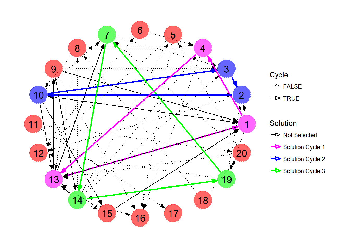
Appendix
The following function performs a depth-first search of the graph, collecting cycles up to a user-specified maximum size. The basic idea is, for some initial node, to visit each of its connections, building up a stack of nodes along the way. We save the stack of nodes if the most recently added node closes a loop with the initial node. If there are no more connections, or the maximum specified cycle size has been reached, we pop the stack and continue. It is essentially Djikstra’s algorithm, with a cap on the depth and a check at each step as to whether the stack represents a closed loop. More details can be found in the code comments.
# Depth-First Search for Cycles in a Network

get_cycles <- function(nodes, edgelist, max_cycle_size){

  cycle_list <- list() # Collect found cycles
  cycles <- 0 # Count cycles

  # Does edge exist in network from 'from' node to 'to' node?
  incidence <- function(from,to){
    return(edgelist %>% filter(X1==from, X2==to) %>% nrow > 0)
  }

  # Retrieve first unvisited child of 'current' node (after 'from' node)
  # Returns -1 if no child found
  get_child <- function(from, current, visited){

    if (from != nodes){
      for (j in (from + 1):nodes){
        if (incidence(current,j) & !visited[j]){
          return(j)
        }
      }
    }

    return(-1)
  }

  # Use stack to store and evaluate current set of nodes
  node_stack <- numeric()

  # Keep note of the first node in the stack (head node)
  current_head_node <- 1

  # Keep track of whether each node has been explored already
  visited <- rep(FALSE, nodes)


  # Iterate over all nodes
  while (current_head_node <= nodes){

    # Place new head node in the stack and mark as visited
    node_stack <- c(node_stack, current_head_node)
    visited[current_head_node] <- TRUE

    # Get the first child of this node
    v <- get_child(current_head_node, current_head_node, visited)

    while(length(node_stack) > 0){

      # If there are no children to explore
      if (v == -1){

        # Pop node from stack
        backtrack_node <- node_stack %>% tail(1)
        node_stack <- node_stack %>% head(-1)

        if (backtrack_node == current_head_node){
          # We've popped the head node from the stack, which is now empty
          # Break from the loop and start a new stack with a new head node
          visited[backtrack_node] <- FALSE
          break
        }

        # Mark the popped node as not visited
        visited[backtrack_node] <- FALSE

        # Get new node from top of stack and get its next unvisited child
        new_top_node <- node_stack %>% tail(1)
        v <- get_child(backtrack_node, new_top_node, visited)


      } else {

        # Place new node on top of stack and mark as visited
        node_stack <- c(node_stack, v)
        visited[v] <- TRUE

        # If this node connects back to the head node, we've found a cycle!
        if (incidence(v,current_head_node)){

          # Check size constraints (may be unnecessary...)
          if (length(node_stack) <= max_cycle_size){

            # Add cycle to list
            cycles <- cycles + 1
            cycle_list[[cycles]] <- node_stack
          }

        }

        if (length(node_stack) >= max_cycle_size){
          # If stack has reached the maximum cycle size, signal that there are no
          # more children to explore
          v <- -1
        } else {
          # Else, grow stack with child of current node
          v <- get_child(current_head_node, v, visited)
        }
      }
    }

    # Advance head node
    current_head_node <- current_head_node + 1

  }

  return(cycle_list)
}