Exploratory Analysis on SNL Episode Ratings
Code and data can be found on Github.
Figured I should chime in here since it’s been… let’s see here… ah, 4 months. I had previously promised to write about some NCAA hockey projects I had been working on. That… will have to wait -_-. In the meantime, let’s look instead at some Saturday Night Live data!
For those not familiar, Saturday Night Live, commonly abbreviated as ‘SNL’, is a comedy-variety show that airs live on NBC on select Saturday nights over the course of a ‘season’, which runs from September through May. SNL first aired in 1975, and is currently airing its 43rd season. Each episode features a celebrity guest host who participates in most of the sketches, along with a musical guest who performs twice over the course of the show.
A simple question came to me after watching a disappointing episode of SNL hosted by Kumail Nanjiani a few weeks ago. This episode just happened to be the third in a sequence of episodes airing over consecutive weeks. Knowing the grueling schedule that SNL writers operate on, I was curious if, as in sports such as hockey, some kind of fatigue, in this case something akin to writer’s block, may impact the quality of an episode.
In this post, I’ll perform exploratory analysis on SNL episode quality to get an idea of whether or not my ‘writer’s fatigue’ hypothesis makes sense. Episode quality will be based on averaged ratings (on a 0-10 scale) of users on IMDb, inspired by previous analyses of TV shows such as ‘The Simpsons’. I’ll note that, while writing this post, I thought the most recent episode hosted by Chance the Rapper was fantastic, and also happened to be the third episode in a stretch of three consecutive weeks of episodes.
I’ll also make clear right at the onset that this post is meant mostly as a fun exercise. There are a number of caveats to using IMDb data, such as the variable number of votes given to each episode, the composition of users that determine the ratings, and the rounding of final ratings to 1 decimal place. SNL ratings in particular are likely highly driven by topical events that occurred around the time of each episode, as well as the quality/notoriety/likability of the host. While a more determined analyst would do well to adjust for these factors, a much more involved cleaning job on the data will likely be required (something for the future perhaps?).
All that being said, let’s get right into it, starting by loading our handy libraries.
library(dplyr)     # Lifeblood of data science
library(rvest)     # Scrape scrape scrape
library(purrr)     # 'map' function
library(zoo)       # 'locf' function for carrying last observation forward
library(lubridate) # Working with dates
library(stringr)   # Working with strings
library(ggplot2)   # Plots
library(ggridges)  # Fancy plots
library(viridis)   # User-friendly color scheme
Scrape, Scrape, Scrape!
For those not interested in the data collection portion of this post, but who still want to play along at home, full data can be found here, and feel free to skip directly to the analysis section.
As is usually the case for any project, the required data will have to be collected in pieces from disparate sources, cleaned separately and merged into a tidy format. First we need the ratings of each episode, which we scrape from IMDb using the read_html, html_nodes, and html_table functions from the rvest package. The main table of interest is the first table collected under the 'table' tag, which we convert to an R data frame.
url <- "http://www.imdb.com/title/tt0072562/epdate" #IMDb URL

raw.ratings <- url %>%
  read_html %>%
  html_nodes('table') %>% # Ratings table is taggeed as 'table'
  html_table(header=F) %>% # Extract tables
  `[[`(1) %>% # Retain first table with ratings
data.frame(stringsAsFactors=F) # Convert to data frame## X1 X2 X3 X4
## 1 # Episode UserRating UserVotes
## 2 1.1 George Carlin/Billy Preston/Janis Ian 7.6 266
## 3 1.2 Paul Simon/Randy Newman/Phoebe Snow 6.5 158
## 4 1.3 Rob Reiner 7.0 129
## 5 1.4 Candice Bergen/Esther Phillips 7.2 126
## 6 1.5 Robert Klein/ABBA, Loudon Wainwright III 6.8 109
## X5
## 1
## 2 1\n2\n3\n4\n5\n6\n7\n8\n9\n10\n\n7.6/10\nX
## 3 1\n2\n3\n4\n5\n6\n7\n8\n9\n10\n\n6.5/10\nX
## 4 1\n2\n3\n4\n5\n6\n7\n8\n9\n10\n\n7.0/10\nX
## 5 1\n2\n3\n4\n5\n6\n7\n8\n9\n10\n\n7.2/10\nX
## 6 1\n2\n3\n4\n5\n6\n7\n8\n9\n10\n\n6.8/10\nXI prefer scraping tables specifying header=F, as the headers of tables on websites tend to be in odd formats that screw up the scraping process (plus I usually end up changing variable names anyway). We remove the first row in our scraped table (which contains the headers we see on the web), then remove the last column of gibberish, and assign our own variable names. From there, we extract the season number from the first column of data, which is the number that appears before the . in that field. Finally, we filter out episodes from the current season (the 43rd season).
# Helper function for extracting the season from the full episode number
extract.season <- function(x){

  token.list <- x %>%
    as.character %>%
    strsplit(split=".", fixed=T) %>% # Season number appears before the '.'
    unlist

  return(as.numeric(token.list[1]))  # Convert to numeric before returning
}

# Clean SNL ratings data
snl.ratings <- raw.ratings %>%
  tail(-1) %>% #  Remove first row
  select(1:4) %>% # Retain first 4 columns
  rename(EpisodeNumber = X1,
         Guests = X2,
         Rating = X3,
         Votes = X4) %>% # Rename variables
  rowwise %>%
  mutate(Season = extract.season(EpisodeNumber)) %>% # Get season number from episode number
  select(Season, Guests, Rating, Votes) %>% # Retain variables
  ungroup %>%
filter(Season < 43) # Not going to consider episodes from the currently airing season## Season Guests Rating Votes
## 1 1 George Carlin/Billy Preston/Janis Ian 7.6 266
## 2 1 Paul Simon/Randy Newman/Phoebe Snow 6.5 158
## 3 1 Rob Reiner 7.0 129
## 4 1 Candice Bergen/Esther Phillips 7.2 126
## 5 1 Robert Klein/ABBA, Loudon Wainwright III 6.8 109
## 6 1 Lily Tomlin 7.2 108So we have our ratings, but if we are to look at how breaks and consecutive runs of episodes affect ratings, we also need the date each episode aired (the ‘airdate’), which is not found in the data we collected. Various sources contain airdate information, including IMDb, though not in a handy table format, meaning a scraper would be quite a bit more tedious to design. Luckily, the airdates happen to be conveniently laid out on Wikipedia, and so we’ll simply go with that.
Tables of airdates, one for each season, are spread across three sections. We collect all tables across all three sections and bind these together. Note that tables in the last section contain some TV ratings information from Nielsen (these estimate number of viewers, not necessarily episode quality), which we omit when combining.
# Helper function for scraping SNL airdate tables from Wikipedia
extract.wiki.table <- function(url){

  raw.data <- url %>%
    read_html %>%
    html_nodes('.wikiepisodetable') %>% # Tables from wikipedia page are tagged with '.wikiepisodetable'
    map(html_table, header=F, fill=T) %>% # Convert scraped tables to data frames
    bind_rows # Bind the set of data frames into one large data frame

  return(raw.data)
}

# Gather and combine raw SNL airdate tables
raw.snl.1 <- extract.wiki.table("https://en.wikipedia.org/wiki/List_of_Saturday_Night_Live_episodes_(seasons_1%E2%80%9315)#Episodes")
raw.snl.2 <- extract.wiki.table("https://en.wikipedia.org/wiki/List_of_Saturday_Night_Live_episodes_(seasons_16%E2%80%9330)#Episodes")
raw.snl.3 <- extract.wiki.table("https://en.wikipedia.org/wiki/List_of_Saturday_Night_Live_episodes#Episodes") %>% select(1:5) # This table has the number of viewers in an extra column, which we leave out

raw.snl.combined <- rbind(raw.snl.1,raw.snl.2,raw.snl.3) # Bind the three data frames together## X X1 X2 X3
## 1 1 No.\noverall No. in\nseason Host
## 2 2 1 1 George Carlin
## 3 3 2 2 Paul Simon
## 4 4 3 3 Rob Reiner
## 5 5 4 4 Candice Bergen
## 6 6 5 5 Robert Klein
## X4
## 1 Musical guest(s)
## 2 Billy Preston & Janis Ian
## 3 Randy Newman, Phoebe Snow, Art Garfunkel & Jessy Dixon Singers
## 4 none
## 5 Esther Phillips
## 6 ABBA & Loudon Wainwright III
## X5
## 1 Original air date
## 2 October 11, 1975 (1975-10-11)
## 3 October 18, 1975 (1975-10-18)
## 4 October 25, 1975 (1975-10-25)
## 5 November 8, 1975 (1975-11-08)
## 6 November 15, 1975 (1975-11-15)Other than removing the website headers collected within the table (conveniently the string ‘Original air date’ appears in each case in the fifth column) and renaming our variables, we extract the airdate from the final column and convert to a more R-friendly format using lubridate.
# Helper function for extracting the correct airdate
extract.airdate <- function(airdate){

  clean.airdate <- airdate %>%
    strsplit(split="(", fixed=T) %>% # Split off date string after '('
    unlist %>% # Convert to vector
    `[`(1) %>% # Extract first element
    trimws %>% # Remove whitespace from beginning and end
    mdy # Convert to simple date format

  return(clean.airdate)
}

# Clean SNL airdate data
snl.airdates <- raw.snl.combined %>%
  rename(EpNumber = X1,
         SeasonEpNumber = X2,
         Host = X3,
         MusicalGuest = X4,
         AirDate = X5) %>% # Rename variables
  filter(AirDate != "Original air date") %>% # Remove rows not pertaining to actual episodes
  mutate(EpNumber = as.numeric(EpNumber),
         SeasonEpNumber = as.numeric(SeasonEpNumber)) %>% # Convert numeric columns
  rowwise %>%
  mutate(AirDate = extract.airdate(AirDate)) %>% # Convert airdate to R friendly format
  ungroup
Notice this data set does not contain the season number, but since we have the episode number within each season, we can extract the first episode of each season and assign its season number, then create a new variable in the original data set with the season number for these episodes and ’NA’s for the rest. We then use the locf function from the zoo package to carry the last observation forward, filling out the season number for the remaning episodes.
# Extract first episodes from each season and assign a season number
first.episodes <- snl.airdates %>%
  filter(SeasonEpNumber == 1) %>%
  mutate(Season = 1:n()) %>%
select(EpNumber, Season)## EpNumber Season
## 1 1 1
## 2 25 2
## 3 47 3
## 4 67 4
## 5 87 5
## 6 107 6snl.airdates <- snl.airdates %>%
left_join(first.episodes, by="EpNumber") %>% # Bind season number based on episode number
mutate(Season = na.locf(Season)) %>% # Carry season number forward to remaining episodes in season
select(Season, SeasonEpNumber, Host, MusicalGuest, AirDate) %>% # Retain variables of interest
filter(Season < 43) # Not going to consider the season currently airing## Season SeasonEpNumber Host
## 1 1 1 George Carlin
## 2 1 2 Paul Simon
## 3 1 3 Rob Reiner
## 4 1 4 Candice Bergen
## 5 1 5 Robert Klein
## 6 1 6 Lily Tomlin
## MusicalGuest
## 1 Billy Preston & Janis Ian
## 2 Randy Newman, Phoebe Snow, Art Garfunkel & Jessy Dixon Singers
## 3 none
## 4 Esther Phillips
## 5 ABBA & Loudon Wainwright III
## 6 Tomlin with Howard Shore & the All Nurse Band
## AirDate
## 1 1975-10-11
## 2 1975-10-18
## 3 1975-10-25
## 4 1975-11-08
## 5 1975-11-15
## 6 1975-11-22Note that, as in the previous case, we omit the episodes from the most recent season.
Merging our Data Sets
So we have two tables of data for what we assume is the same set of episodes. Simply bind the columns together and we’re good to go, right? Well, not so fast…
snl.airdates.season.counts <- snl.airdates %>%
  group_by(Season) %>%
  summarize(N1=n()) %>%
  arrange(Season)

snl.ratings.season.counts <- snl.ratings %>%
  group_by(Season) %>%
  summarize(N2=n()) %>%
  arrange(Season)

snl.airdates.season.counts %>%
  left_join(snl.ratings.season.counts, by="Season") %>%
  mutate(SameCounts = N1==N2) %>%
filter(!SameCounts)## # A tibble: 2 x 4
## Season N1 N2 SameCounts
## <int> <int> <int> <lgl>
## 1 2 22 23 FALSE
## 2 10 17 18 FALSEIt seems the number of episodes in each seasons don’t line up exactly; there are extra episodes in the ratings dataset for Seasons 2 and 10.
Typically, in a larger data setting, one would employ some kind of fuzzy matching scheme to match the Host field from the airdate dataset and the Guest field from the ratings dataset (especially since we can’t generally guarantee that the correct order of data points has been preserved). Since the data here is not particularly large, and there appears to only be two errors, we will inspect the situation manually.
# Seasons 2 and 10 have an extra episode in the ratings data set, let's find them!
snl.airdates %>%
  filter(Season == 2) %>%
  .$Host
## [1] "Lily Tomlin" "Norman Lear" "Eric Idle"
## [4] "Karen Black" "Steve Martin" "Buck Henry"
## [7] "Dick Cavett" "Paul Simon" "Jodie Foster"
## [10] "Candice Bergen" "Ralph Nader" "Ruth Gordon"
## [13] "Fran Tarkenton" "Steve Martin" "Sissy Spacek"
## [16] "Broderick Crawford" "Jack Burns" "Julian Bond"
## [19] "Elliott Gould" "Eric Idle" "Shelley Duvall"
## [22] "Buck Henry"snl.ratings %>%
filter(Season == 2) %>%
.$Guests ## [1] "Lily Tomlin/James Taylor"
## [2] "Norman Lear/Boz Scaggs"
## [3] "Eric Idle/Joe Cocker/Stuff"
## [4] "Karen Black/John Prine"
## [5] "Steve Martin/Kinky Friedman"
## [6] "Buck Henry/The Band"
## [7] "Dick Cavett/Ry Cooder"
## [8] "Paul Simon/George Harrison"
## [9] "Jodie Foster/Brian Wilson"
## [10] "Candice Bergen/Frank Zappa"
## [11] "Ralph Nader/George Benson"
## [12] "Ruth Gordon/Chuck Berry"
## [13] "Fran Tarkenton/Leo Sayer, Donnie Harper and the Voices of Tomorrow"
## [14] "Live from Mardi Gras"
## [15] "Steve Martin/The Kinks"
## [16] "Sissy Spacek/Richard Baskin"
## [17] "Broderick Crawford/Levon Helm/Dr. John/The Meters"
## [18] "Jack Burns/Santana"
## [19] "Julian Bond/Tom Waits, Brick"
## [20] "Elliott Gould/Kate & Anna McGarrigle/Roslyn Kind"
## [21] "Eric Idle/Neil Innes"
## [22] "Shelley Duvall/Joan Armatrading"
## [23] "Buck Henry/Jennifer Warnes/Kenny Vance"The episode ‘Live from Mardi Gras’ appears in the ratings data but not the airdate data.
snl.airdates %>%
  filter(Season == 10) %>%
  .$Host
## [1] "(none)" "Bob Uecker" "Jesse Jackson"
## [4] "Michael McKean" "George Carlin" "Ed Asner"
## [7] "Ed Begley, Jr." "Ringo Starr" "Eddie Murphy"
## [10] "Kathleen Turner" "Roy Scheider" "Alex Karras"
## [13] "Harry Anderson" "Pamela Sue Martin" "Mr. THulk Hogan"
## [16] "Christopher Reeve" "Howard Cosell"snl.airdates %>%
filter(Season == 10, SeasonEpNumber == 1) %>%
.$MusicalGuest## [1] "Thompson Twins"snl.ratings %>%
filter(Season == 10) %>%
.$Guests ## [1] "Thompson Twins"
## [2] "Bob Uecker/Peter Wolf"
## [3] "Jesse Jackson/Andrae Crouch, Wintley Phipps"
## [4] "Michael McKean/Chaka Khan/The Folksmen"
## [5] "George Carlin/Frankie Goes to Hollywood"
## [6] "Ed Asner/The Kinks"
## [7] "Ed Begley Jr/Billy Squier"
## [8] "Ringo Starr/Herbie Hancock"
## [9] "Eddie Murphy/Robert Plant & The Honeydrippers"
## [10] "Kathleen Turner/John Waite"
## [11] "Roy Scheider/Billy Ocean"
## [12] "Alex Karras/Tina Turner"
## [13] "Harry Anderson/Bryan Adams"
## [14] "Pamela Sue Martin/Power Station"
## [15] "SNL Film Festival"
## [16] "Mr. T and Hulk Hogan/The Commodores"
## [17] "Christopher Reeve/Santana"
## [18] "Howard Cosell/Greg Kihn"The extra season 10 episode in the ratings dataset is ‘SNL Film Festival’. Note that while the host of the season premiere is listed as ‘(none)’ in the airdate dataset, the musical guest (‘Thompson Twins’) matches the Guest field from the ratings dataset (in some SNL episodes, the host doubles as the musical guest).
We filter out these two extra episodes, and then bind the two datasets together.
snl.ratings <- snl.ratings %>%
  filter(!(Guests %in% c("Live from Mardi Gras","SNL Film Festival")))
# Combine data frames
snl.data <- cbind(snl.airdates, snl.ratings %>% select(-Season)) %>%
select(Season,SeasonEpNumber,Guests,Host,MusicalGuest,AirDate,Rating,Votes)Below are the episodes were the Host field string (originally from the airdate dataset) is not detected within the Guest field string (originally from the ratings dataset. I leave it to you to check that there are no issues other than typos (e.g. ‘Donald Pleasance’ vs. ‘Donald Pleasence’), improper capitalizations (e.g. ‘Elle MacPherson’ vs. ‘Elle Macpherson’), non-matching abbreviations (e.g. ‘Louis Gossett Jr’ vs. ‘Louis Gossett Jr.’), alternate names (e.g. ‘Tom & Dick Smothers’ vs. ‘The Smothers Brothers’), spacing issues (e.g. O.J. Simpson vs. O. J. Simpson) or combined hosts/musical guests that only appear in one column and not the other. Note that I’ve truncated the strings to make them easier to display.
# Quick sanity check, which episodes don't match hosts between data sets?
# Does the 'Host' from the Airdate data appear in the 'Guest' from the Ratings data?
snl.data %>%
  mutate(MatchDetected = str_detect(Guests,fixed(Host))) %>%
  filter(!MatchDetected) %>%
  mutate(Guests = str_sub(Guests,0,20),
         Host = str_sub(Host,0,20),
         MusicalGuest = str_sub(MusicalGuest,0,20)) %>%
select(Season,Guests,Host,MusicalGuest)## Season Guests Host MusicalGuest
## 1 3 O.J. Simpson/Ashford O. J. Simpson Ashford and Simpson
## 2 5 Paul Simon, James Ta none Paul SimonJames Tayl
## 3 5 Richard Benjamin, Pa Richard BenjaminPaul The Grateful Dead
## 4 6 Jr. Walker & the All none Jr. Walker & the All
## 5 7 Rod Stewart (none) Rod Stewart
## 6 7 Donald Pleasance/Fea Donald Pleasence Fear
## 7 8 Louis Gossett Jr/Geo Louis Gossett, Jr. George Thorogood & t
## 8 8 Tom & Dick Smothers/ The Smothers Brother Laura Branigan
## 9 8 Rick Moranis and Dav Rick MoranisDave Tho The Bus Boys
## 10 8 Beau and Jeff Bridge Beau BridgesJeff Bri Randy Newman
## 11 8 Robert Guilaume/Dura Robert Guillaume Duran Duran
## 12 9 Danny DeVito & Rhea Danny DeVito & Rhea Eddy Grant
## 13 9 Father Guido Sarducc Father Guido Sarducc Huey Lewis and the N
## 14 9 Billy Crystal/Ed Koc Billy Crystal, Ed Ko The Cars
## 15 10 Thompson Twins (none) Thompson Twins
## 16 10 Ed Begley Jr/Billy S Ed Begley, Jr. Billy Squier
## 17 10 Mr. T and Hulk Hogan Mr. THulk Hogan The Commodores
## 18 11 Pee Wee Herman/Queen Paul Reubens as Pee- Queen Ida & the Bon
## 19 11 George Wendt and Fra George WendtFrancis Philip Glass
## 20 11 Catherine Oxenberg a Catherine OxenbergPa Paul SimonLadysmith
## 21 11 Anjelica Huston and Anjelica HustonBilly George ClintonParlia
## 22 12 Chevy Chase/Steve Ma Chevy Chase, Steve M Randy Newman
## 23 12 Walter Payton & Joe Joe MontanaWalter Pa Deborah Harry
## 24 17 Hammer MC Hammer MC Hammer
## 25 17 Jason Priestly/Teena Jason Priestley Teenage Fanclub
## 26 17 Roseanne & Tom Arnol Roseanne ArnoldTom A Red Hot Chili Pepper
## 27 19 Shannon Doherty/Cypr Shannen Doherty Cypress Hill
## 28 19 Alec Baldwin & Kim B Alec Baldwin and Kim UB40
## 29 21 Elle MacPherson/Stin Elle Macpherson Sting
## 30 22 Robert Downey Jr/Fio Robert Downey, Jr. Fiona Apple
## 31 22 Pamela Lee/Rollins B Pamela Anderson Rollins Band
## 32 23 Rudy Giuliani/Sarah Rudolph Giuliani Sarah McLachlan
## 33 24 Cuba Gooding, Jr./Ri Cuba Gooding Jr. Ricky Martin
## 34 25 The Rock/AC/DC The Rock (Dwayne Joh AC/DC
## 35 27 Ellen Degeneres/No D Ellen DeGeneres No Doubt
## 36 27 The Rock/Andrew W.K. Dwayne Johnson Andrew W.K.
## 37 29 Jessica Simpson and Jessica Simpson & Ni G-Unit
## 38 29 Mary-Kate & Ashley O Mary-Kate and Ashley J-Kwon
## 39 40 J.K. Simmons/D'Angel J. K. Simmons D'AngeloSNL Ratings Distributions
Alright, we have our data, now let’s make some charts! First let’s take a quick look at ratings curves by season. We use the excellent ggridges package, by Claus O. Wilke (available from CRAN), to display the large number of density curves (note that you may have heard of this package by another name). I also use the viridis package to display the median episode rating for each season by a user-friendly color.
# Extract median episode rating for each season
median.ratings <- snl.data %>%
  group_by(Season) %>%
  summarize(MedianRating = median(Rating))

# Merge medians to SNL data
snl.data <- snl.data %>%
  left_join(median.ratings, by="Season")

# Plot rating densities
ggplot(data=snl.data, aes(x=Rating, y=as.factor(Season), fill=MedianRating)) +
  geom_density_ridges(alpha=0.7, rel_min_height=0.01) +
  scale_fill_viridis(name = "Median Rating") +
  scale_y_discrete(position="right") +
  theme_bw(16) +
  xlim(0,10) +
  xlab("Rating") +
  ylab("Season") +
  annotate("text",x=5,y=20,col="red",label="@mathieubray 2017",
           alpha=0.15,cex=15,fontface="bold",angle=30) +
  ggtitle("SNL Ratings Density by Season", subtitle = "Color represents median episode rating from the given season. Data from imdb.com")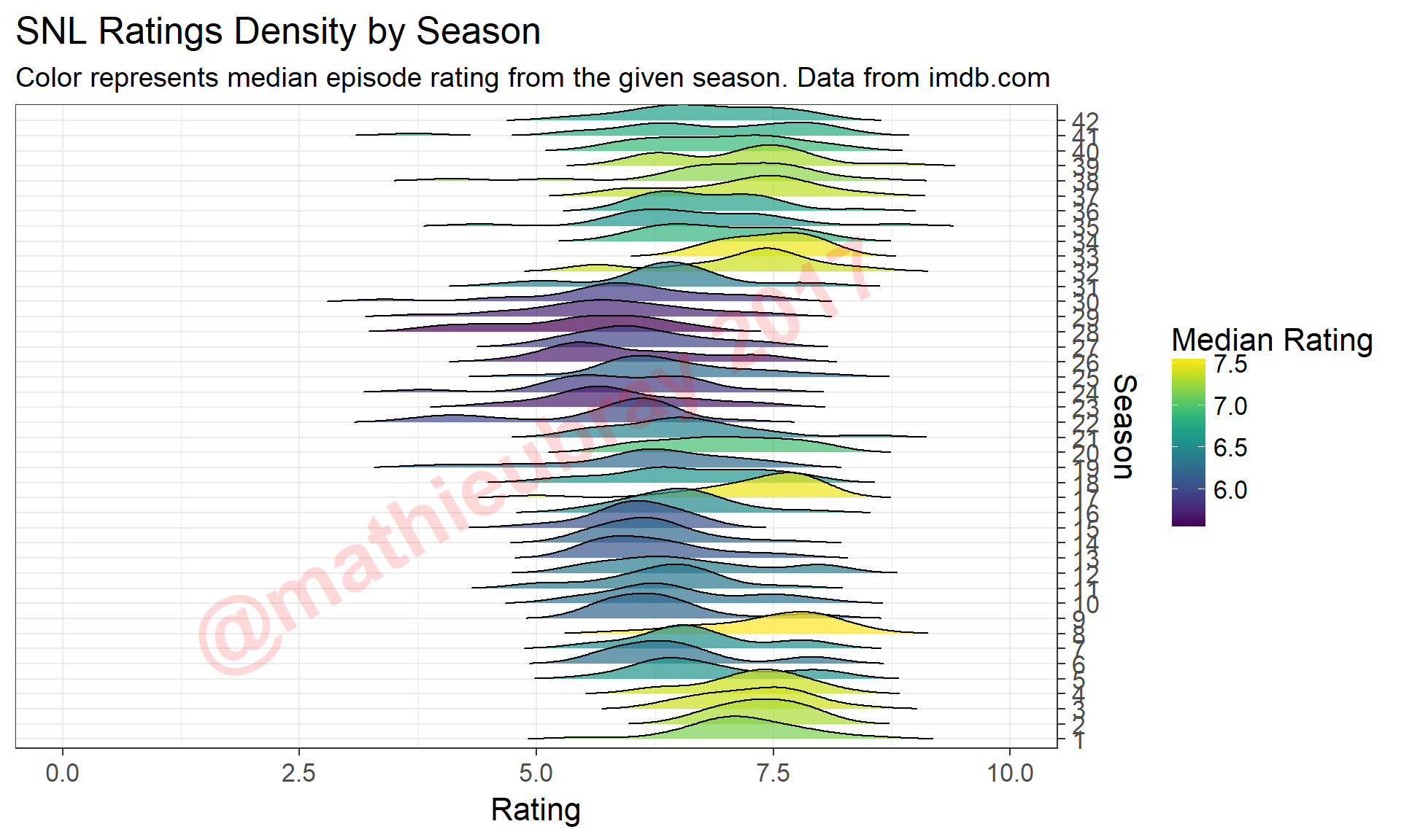
This chart gives a nice snapshot of viewer’s impressions of SNL over the years, with strong early seasons followed by a comparatively mediocre stretch from Seasons 9-16 (corresponding to 1983-1990), and another slightly worse stretch around Season 22 to Season 30 (1996-2004). While recent seasons appear to be more favorably rated in general, there does not seem to be much evidence to suggest any major SNL renaissance (which one would assume if we look at the number of Emmys earned last season).
Check out that rough patch in Season 41 where the density perks up far to the left of the main ratings curve. Tough to tell what may have caused that…
snl.data %>%
  filter(Season==41, Rating < 4.0) %>%
select(Season, SeasonEpNumber, Host, AirDate, Rating, Votes)# One of the least popular episodes## Season SeasonEpNumber Host AirDate Rating Votes
## 1 41 4 Donald Trump 2015-11-07 3.7 492I’ll reiterate here that the IMDb ratings are reported as the average of ratings on a 0-10 scale. I should note that the number of votes tend to be high for recent episodes as well as early episodes, while episodes from most of the other seasons have comparatively much fewer votes.
mean.votes <- snl.data %>%
  group_by(Season) %>%
  summarize(MeanVotes = mean(Votes))

snl.data <- snl.data %>%
  left_join(mean.votes, by="Season")

ggplot(data=snl.data, aes(x=as.factor(Season), y=Votes, color = MeanVotes)) +
  scale_color_viridis(name = "Mean Number of Votes", direction=-1) +
  geom_boxplot(size=0.75) +
  xlab("Season") +
  theme_bw(16) +
  coord_flip() +
  annotate("text",x=21,y=250,col="red",label="@mathieubray 2017",
           alpha=0.15,cex=12,fontface="bold",angle=30) +
  ggtitle("Number of Votes for SNL Rating is Not Consistent Season to Season",
          subtitle="Color represents mean number of votes by season. Data from imdb.com" )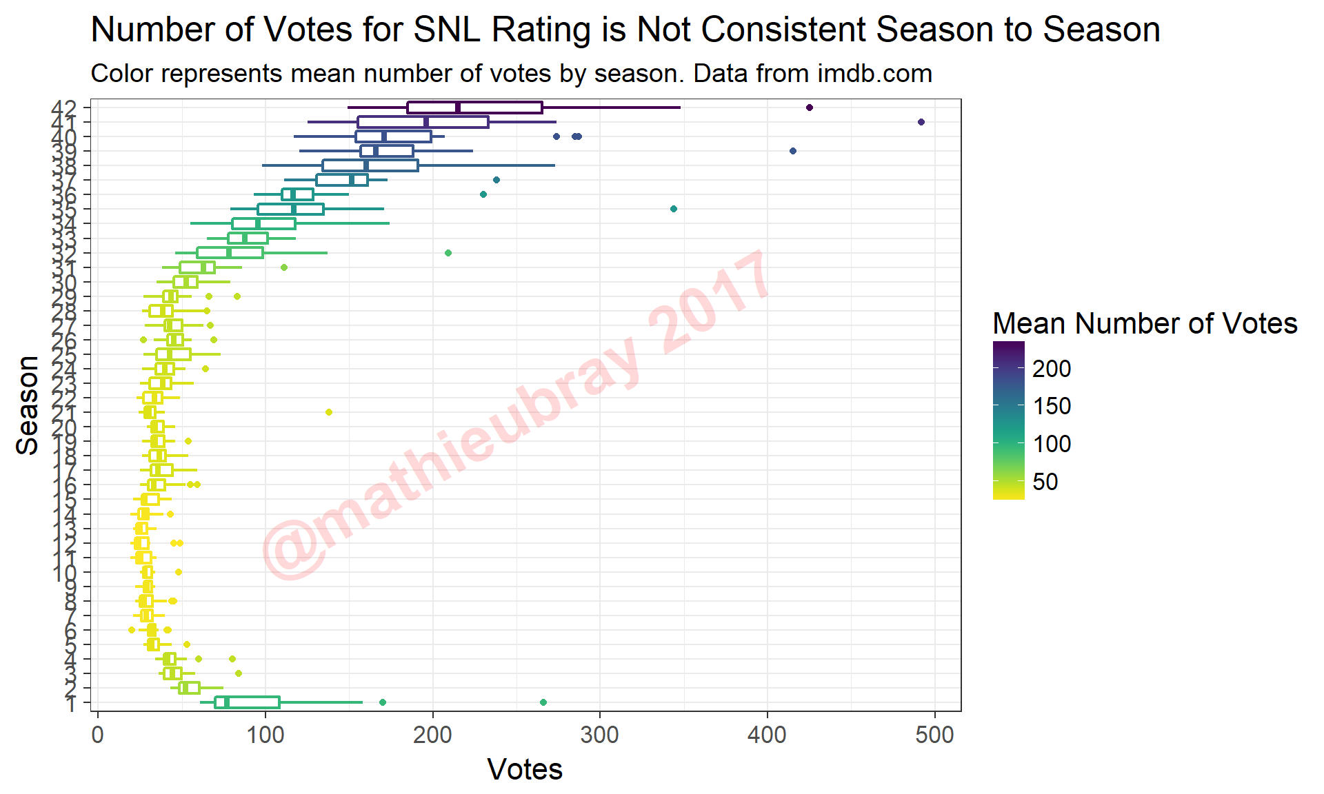
The overall distribution of ratings is shown below, as both a histogram (recall that ratings are collected rounded to 1 decimal place, effectively discretizing the data), as well as a density curve.
ggplot(data=snl.data, aes(Rating)) +
  geom_histogram(stat="count",alpha=0.8,fill="blue") +
  theme_bw(16) +
  xlim(0,10) +
  ylim(0,50) +
  xlab("Rating") +
  ylab("Number of Episodes") +
  annotate("text",x=5,y=25,col="red",label="@mathieubray 2017",
           alpha=0.15,cex=15,fontface="bold",angle=30) +
  ggtitle("SNL Ratings Histogram",
          subtitle="Data from imdb.com" )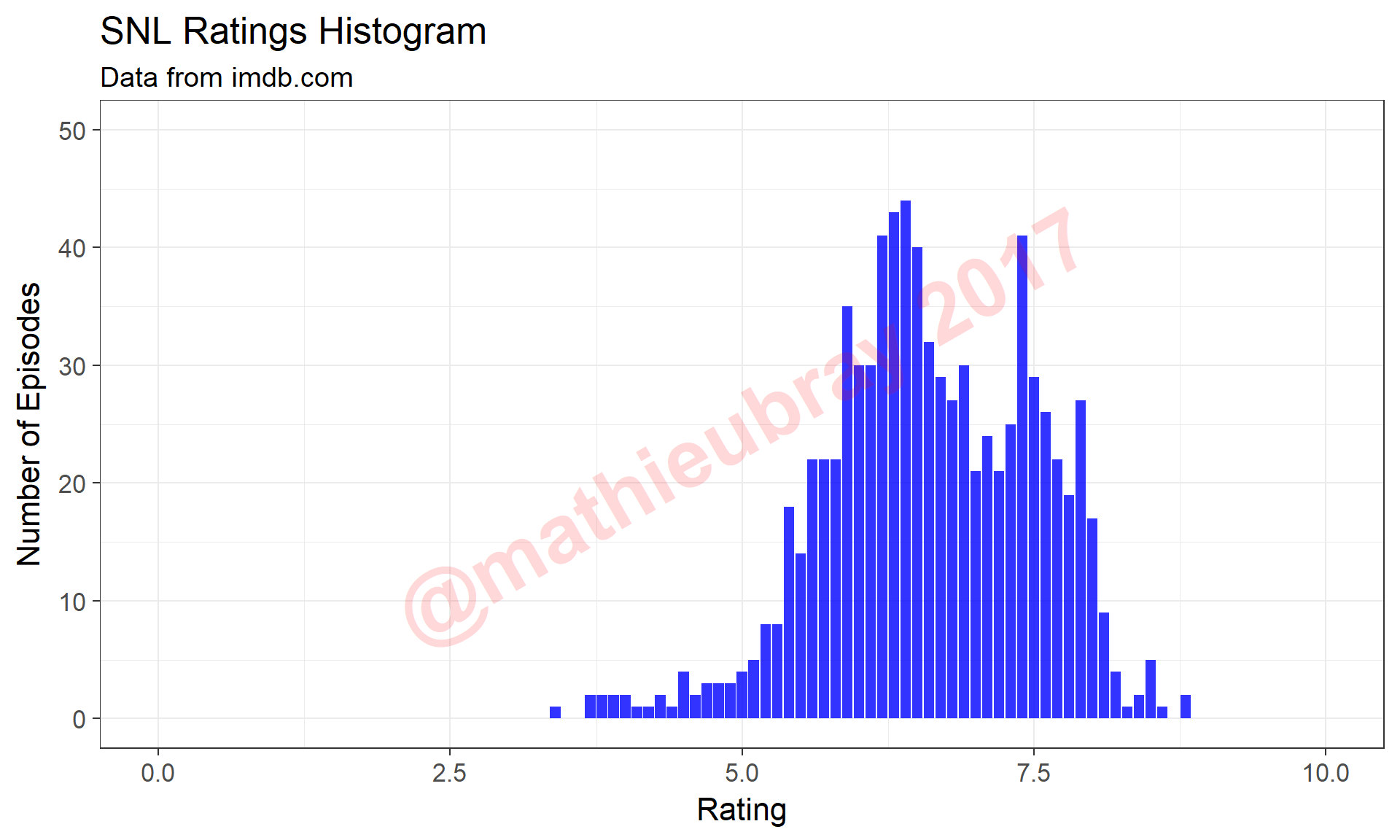
ggplot(data=snl.data, aes(x=Rating)) +
  geom_density(alpha=0.5, fill="blue") +
  theme_bw(16) +
  xlim(0,10) +
  xlab("Rating") +
  ylab("Density") +
  annotate("text",x=5,y=0.25,col="red",label="@mathieubray 2017",
           alpha=0.15,cex=15,fontface="bold",angle=30) +
  ggtitle("SNL Ratings Density",
          subtitle="Data from imdb.com" )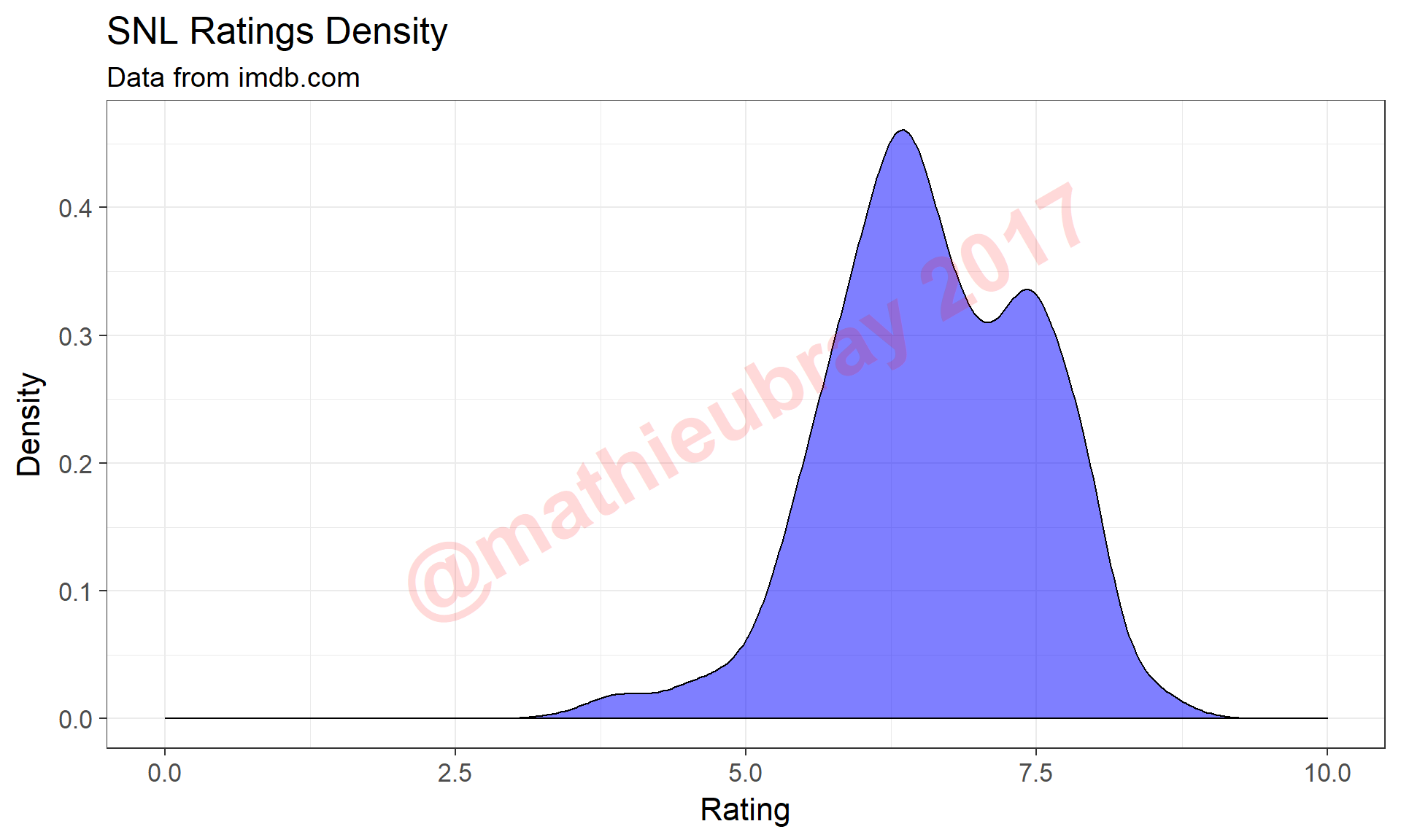
We observe a bimodal density curve with most episodes earning ratings around 6.0 (‘mediocre’ episodes), or around 7.5 (‘good-great’ episodes). We continue to use densities going forward, mostly based on their elegance and ease of qualitative interpretation.
SNL Ratings Based on Number of Weeks Between Episodes
We are interested in observing whether some kind of ‘writer fatigue’ may affect the quality of SNL episodes. First, we will calculate for each episode the number of weeks since the previous episode, a.k.a. the break betwen each episode. This can be achieved using the lag function (to collect in a separate variable the airdate of the episode previous to each episode), and the as.period function from the lubridate package, to extract the difference in days between two airdates, which we then convert to a number of weeks. A snippet of the data with the new column is shown below.
### Ratings based on number of weeks since last episode

# Add in the number of weeks since the last episode
snl.data.enhanced <- snl.data %>%
  mutate(PreviousAirDate = lag(AirDate), # Get airdate of previous episode
         WeeksSinceLastEpisode = as.period(AirDate - PreviousAirDate)@day / 7) %>% # Calculate number of weeks since last episode
  select(-PreviousAirDate)
snl.data.enhanced %>%
filter(Season==42) %>%
select(SeasonEpNumber,Host,AirDate,WeeksSinceLastEpisode) %>%
head(10)## SeasonEpNumber Host AirDate WeeksSinceLastEpisode
## 1 1 Margot Robbie 2016-10-01 19
## 2 2 Lin-Manuel Miranda 2016-10-08 1
## 3 3 Emily Blunt 2016-10-15 1
## 4 4 Tom Hanks 2016-10-22 1
## 5 5 Benedict Cumberbatch 2016-11-05 2
## 6 6 Dave Chappelle 2016-11-12 1
## 7 7 Kristen Wiig 2016-11-19 1
## 8 8 Emma Stone 2016-12-03 2
## 9 9 John Cena 2016-12-10 1
## 10 10 Casey Affleck 2016-12-17 1Note that the season premiere will always have a large break (SNL does not air over the summer). Let’s look at the distribution of break lengths.
# Standardize these weeks into categories
snl.data.enhanced %>%
  group_by(WeeksSinceLastEpisode) %>%
count## # A tibble: 18 x 2
## # Groups: WeeksSinceLastEpisode [18]
## WeeksSinceLastEpisode n
## <dbl> <int>
## 1 1 481
## 2 2 132
## 3 3 117
## 4 4 41
## 5 5 10
## 6 6 4
## 7 7 1
## 8 8 1
## 9 16 1
## 10 17 2
## 11 18 3
## 12 19 17
## 13 20 11
## 14 21 3
## 15 25 2
## 16 30 1
## 17 32 1
## 18 NA 1(The NA above is due to the first episode not having a previous episode from which to calculate the number of weeks since the last episode). We discretize our variable, using the case_when function from the dplyr package (which I first learned from here, along with some other neat dplyr tricks), designating any break longer than 4 weeks as 4+ to balance the categories.
snl.data.enhanced <- snl.data.enhanced %>%
  mutate(WeeksCat = case_when(.$WeeksSinceLastEpisode >= 4 ~ "4+",
                            is.na(WeeksSinceLastEpisode) ~ "4+",
                            TRUE ~ as.character(WeeksSinceLastEpisode))) # Truncate at 4+ weeks break

snl.data.enhanced %>%
  group_by(WeeksCat) %>%
count## # A tibble: 4 x 2
## # Groups: WeeksCat [4]
## WeeksCat n
## <chr> <int>
## 1 1 481
## 2 2 132
## 3 3 117
## 4 4+ 99The ratings densities for each group of break lengths are shown below, with the overall rating density in the background in grey.
# Plot distributions based on number of weeks between episodes
ggplot(data=snl.data.enhanced, aes(x=Rating, fill=WeeksCat)) +
  geom_density(data = snl.data.enhanced %>% select(-WeeksCat), fill = "darkgrey") +
  geom_density(alpha = 0.5) +
  facet_wrap(~WeeksCat) +
  scale_fill_viridis(name="Weeks Since Last Episode",discrete=T) +
  theme_bw(16) +
  xlim(0,10) +
  ylim(0,0.62) +
  xlab("Rating") +
  ylab("Density") +
  annotate("text",x=5,y=0.31,col="red",label="@mathieubray 2017",
           alpha=0.15,cex=6,fontface="bold",angle=30) +
  ggtitle("Does the Break Before an SNL Episode Affect its Rating?",
          subtitle="Grey curves represent overall ratings density. Data from imdb.com" )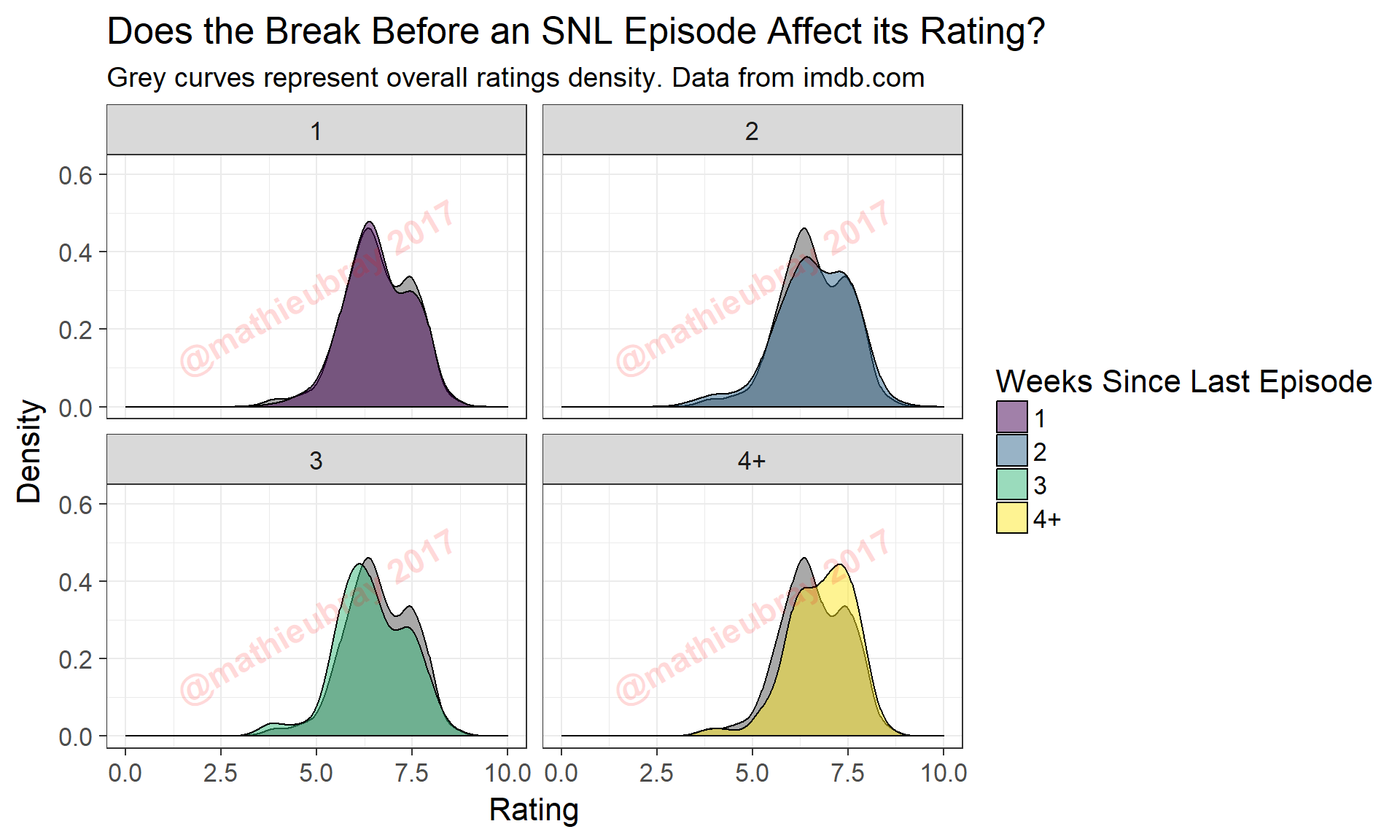
Some takeaways from this set of charts:
- The ‘good-great’ mode is lower for episodes with no break (equivalently, 1 week since last episode)
- Episodes with a week break prior (equivalently, 2 weeks since last episode) see a more even distribution of episode ratings
- For episodes with long breaks prior to air, the distribution skews much higher toward ‘good-great’
This seems to lend evidence to support the fatigue hypothesis, though there are a few other factors we should probably keep in mind. Let’s look at episodes written with at least a week break versus those without.
snl.data.enhanced <- snl.data.enhanced %>%
  mutate(FreshEpisode = WeeksCat != "1") # Mark whether the episode is 'fresh' (at least 1 week break between episodes)

snl.data.enhanced %>%
  group_by(FreshEpisode) %>%
count## # A tibble: 2 x 2
## # Groups: FreshEpisode [2]
## FreshEpisode n
## <lgl> <int>
## 1 FALSE 481
## 2 TRUE 348ggplot(data=snl.data.enhanced, aes(x=Rating, fill=FreshEpisode)) +
geom_density(alpha=0.5) +
scale_fill_viridis(discrete=T, name = "", labels=c("No Break","Break")) +
theme_bw(16) +
xlim(0,10) +
ylim(0,0.5) +
xlab("Rating") +
ylab("Density") +
annotate("text",x=5,y=0.25,col="red",label="@mathieubray 2017",
alpha=0.15,cex=15,fontface="bold",angle=30) +
ggtitle("Are Ratings Affected by Whether an Episode Airs After a Break?",
subtitle="Color represents whether episodes are the first of their seasons ('Premiere') or not ('Not Premiere').\nData from imdb.com" )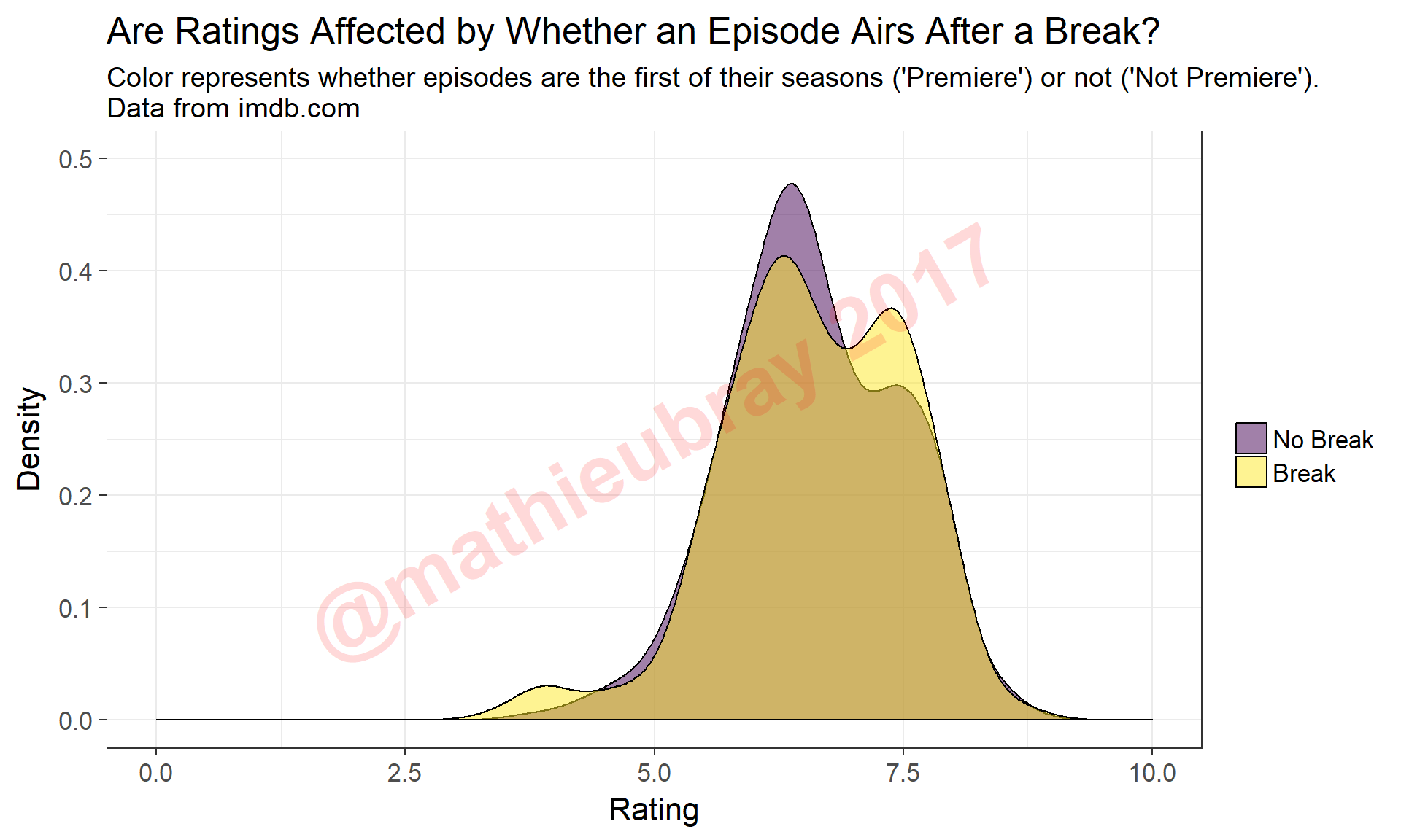
The ‘No Break’ curve is equivalent to the top-left graph from the previous chart. We once again observe a bimodal distribution for episodes that aired with a break, though with fewer ‘medicore’ episodes and more ‘good-great’ episodes. It is interesting that we also observe a small third cluster of very poorly rated episodes among episodes that aired with a break.
Most of the episodes with at least 4 weeks of break are season premieres, ostensibly with a full summer of ideas fresh in the writers’ minds. Let’s look at the distribution of ratings for season premieres versus non-season premieres.
snl.data.enhanced <- snl.data.enhanced %>%
  mutate(Premiere = SeasonEpNumber == 1)

snl.data.enhanced %>%
  group_by(Premiere) %>%
count## # A tibble: 2 x 2
## # Groups: Premiere [2]
## Premiere n
## <lgl> <int>
## 1 FALSE 787
## 2 TRUE 42With the obvious caveat that there are only 42 season premieres with which to draw the density, the two curves are shown below.
ggplot(data=snl.data.enhanced, aes(x=Rating, fill=Premiere)) +
  geom_density(position="identity",alpha=0.5) +
  scale_fill_viridis(discrete=T, name = "", labels=c("Not Premiere","Premiere")) +
  theme_bw(16) +
  xlim(0,10) +
  ylim(0,0.5) +
  xlab("Rating") +
  ylab("Density") +
  annotate("text",x=5,y=0.25,col="red",label="@mathieubray 2017",
           alpha=0.15,cex=15,fontface="bold",angle=30) +
  ggtitle("Are Ratings Affected by Whether an Episode is a Season Premiere?",
          subtitle="Color represents whether episodes are the first of their seasons ('Premiere') or not ('Not Premiere').\nData from imdb.com" )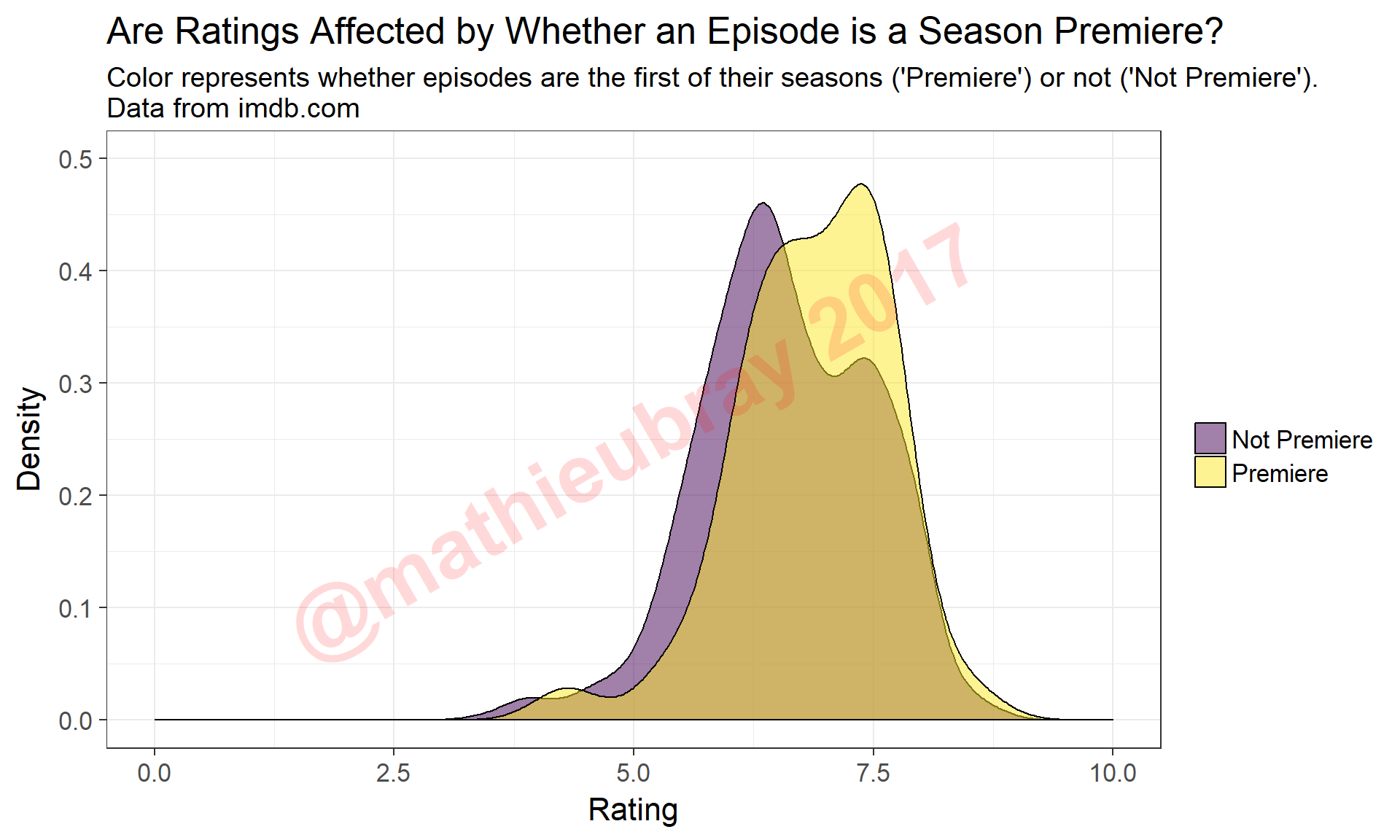
Season premieres appear in general to be very highly rated compared to other episodes.
SNL Ratings Based on Consecutive Episode Sequences
Similar the length of the break prior to each episode, we can also look at the sequence of consecutive episodes and how that affects episode ratings. Episodes that air at the end of a sequence of consecutive episodes may well suffer in quality compared to those at the beginning of the sequence (i.e. those that aired after at least a week break).
The code to determine the placement of each episode within a sequence of consecutive episodes is included below. I used a ‘for’ loop here (gasp!), since I couldn’t quite figure out how to do this effectively in a more R-friendly way. If anyone has any suggestions, shoot me a line in the comments or on the Twitters.
num.episodes <- length(snl.data.enhanced$FreshEpisode)

consecutive.weeks <- numeric(num.episodes)
counter <- 1

for (i in 1:num.episodes){

  if (snl.data.enhanced$FreshEpisode[i]){ # If the episode is fresh
    counter <- 1 # Reset counter
  } else {
    consecutive.weeks[i] <- counter # For episode i, counter = number of episodes in consecutive weeks
    counter <- counter + 1 # Augment counter
  }
}

snl.data.enhanced$ConsecutiveWeeks <- consecutive.weeks

snl.data.enhanced %>%
  filter(Season==42) %>%
  select(SeasonEpNumber,Host,AirDate,ConsecutiveWeeks) %>%
head(10)## SeasonEpNumber Host AirDate ConsecutiveWeeks
## 1 1 Margot Robbie 2016-10-01 0
## 2 2 Lin-Manuel Miranda 2016-10-08 1
## 3 3 Emily Blunt 2016-10-15 2
## 4 4 Tom Hanks 2016-10-22 3
## 5 5 Benedict Cumberbatch 2016-11-05 0
## 6 6 Dave Chappelle 2016-11-12 1
## 7 7 Kristen Wiig 2016-11-19 2
## 8 8 Emma Stone 2016-12-03 0
## 9 9 John Cena 2016-12-10 1
## 10 10 Casey Affleck 2016-12-17 2We do a quick check of the counts of the number of episodes aired consecutively prior to each episode.
snl.data.enhanced %>%
  group_by(ConsecutiveWeeks) %>%
count## # A tibble: 4 x 2
## # Groups: ConsecutiveWeeks [4]
## ConsecutiveWeeks n
## <dbl> <int>
## 1 0 348
## 2 1 332
## 3 2 142
## 4 3 7The longest string of episodes airing on consecutive weeks is 4 (i.e. episodes with 3 consecutive episodes prior), and there are only 7 such instances. We thus categorize the variable and include any episode with 3 consecutive episodes prior into the ‘2-3’ category. Densities are plotted below.
snl.data.enhanced <- snl.data.enhanced %>%
  mutate(ConsecutiveCat = case_when(.$ConsecutiveWeeks >= 2 ~ "2-3",
                          is.na(ConsecutiveWeeks) ~ "2-3",
TRUE ~ as.character(ConsecutiveWeeks)))ggplot(data=snl.data.enhanced, aes(x=Rating, fill=ConsecutiveCat)) +
geom_density(data = snl.data.enhanced %>% select(-ConsecutiveCat), fill = "darkgrey") +
geom_density(alpha=0.7) +
facet_wrap(~ConsecutiveCat) +
scale_fill_viridis(name = "Number of Consecutive Episodes Prior", discrete=T) +
theme_bw(16) +
xlim(0,10) +
xlab("Rating") +
ylab("Density") +
annotate("text",x=5,y=0.31,col="red",label="@mathieubray 2017",
alpha=0.15,cex=6,fontface="bold",angle=30) +
theme(legend.position = "bottom") +
ggtitle("Do Long Sequences of Episodes Affect Ratings?",
subtitle="Grey curves represent overall ratings density. Data from imdb.com" )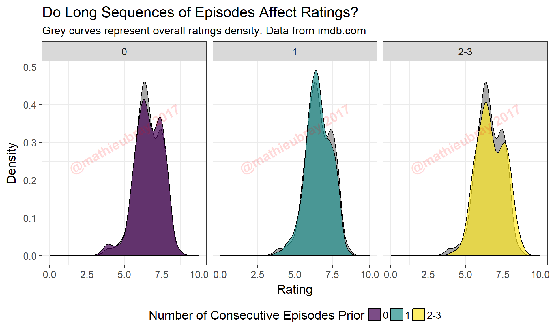
The leftmost panel is equivalent to the ‘Break’ curve shown previously. Episodes that aired as the second in a sequence of episodes (middle panel) see slightly more ‘mediocre’ episodes and slightly fewer ‘good-great’ episodes. The rightmost panel, which include episodes airing at the end of a long sequence of episodes, appears to be more spread out, with dips in both of the main modes. While interesting, there may be more at play here. For example, it may make a difference if, for example, the episode is the second in a long sequence of consecutive episodes versus the second episode in a sequence of two consecutive episodes. Perhaps a question for another day…
That’s about as much effort as I’m willing to put into this right now. As I said, not super deep, though I have a few ideas on how one can augment this data for some possible additional insights. Anyway, that’s it for now. Tune in for more fun stuff from me, and Live… from Ann Arbor… it’s Saturday Night! (spent staying in and procrastinating on actual work by writing this instead!)